Using Otsu’s method to generate data for training of deep learning image segmentation models

Clemens Wolff

May 17th, 20180 0

Background

Partnering with Microsoft, golf performance tracking startup Arccos has set out to use artificial intelligence and machine learning technology to build apps that help golfers step up their game. Last year, they gifted golfers a new ace in the hole – their own “virtual caddie” app, powered by Microsoft’s cloud and machine learning.

Accompanying you on the links and crunching data collected on your personal swing history, the 61 million shots hit by other Arccos users, and 386 million geotagged data points from 40,000 courses, the Arccos virtual caddie provides sage advice on each shot, just like a real caddie. To deliver all this insight, the Arccos virtual caddie needed to understand the playable and non-playable areas of a golf course. Understanding course layout at the necessary granularity requires sophisticated image segmentation, built on deep learning techniques over vast amounts of training data.

That’s where our team came in: in March 2018 we partnered with Arccos to develop a method for rapidly pre-labeling training data for image segmentation models. The auto-labeling technique introduced in this article eliminates the need to painstakingly hand-annotate every pixel of interest in an image. Instead, our technique enables annotators to label training data for image segmentation algorithms rapidly.

Screenshot of Arccos’ virtual caddie application. If the caddie knows that there is a tree or some other non-playable obstacle between the golfer and the green (A and B), it can suggest an alternate path to the green.

By making more training data available, we generalized Arccos’ deep learning model and thus improved the virtual caddie’s performance. The approach we developed applies to any image segmentation task that aims to identify a subset of visually distinct pixels in an image.

Challenges and Objectives

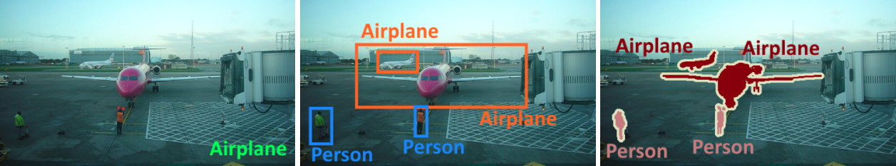
As opposed to image classification – i.e., “what is this image?” – and object detection – i.e., “where are the bounding boxes of objects in this image?” – image segmentation is the task of finding the full complex shape of objects in a picture – i.e., “what is the exact pixel mask of objects in this image?”

Comparison of the three main image-based machine learning tasks: image classification (left), object detection (center) and image segmentation (right).

To create training data for image segmentation tasks, complex shapes in images must be precisely outlined. Compared to assigning tags for image classification or drawing bounding boxes for object detection, the process of creating training data for image segmentation is very time-consuming and prone to annotator error. This annotation process was a major blocker for Arccos: the time expense to create precise masks led to small training sets for their playable-area detector. Moreover, errors in the annotation process add noise to the labeled dataset and hurt the overall performance of the models.

In the remainder of this article, we demonstrate the use of traditional computer vision techniques for pre-labeling training data for image segmentation tasks. Instead of requiring a human annotator to spend many minutes creating the segmentation masks, our technique enables the annotator to verify the segmentation masks in a matter of seconds.

Specifically, we explore the use of thresholding methods in Python and OpenCV to segment the playable area on a golf course given a satellite image. The approaches outlined in this article can be leveraged and adapted to generate training data for any image segmentation task.

Example of a satellite image of a golf course (left) with a human-created mask in orange denoting the non-playable area (right). It takes about 5 minutes to manually create the mask on the right, which makes training data labeling very expensive. However, verifying that the mask is of reasonable quality can be done in about 10 seconds.

Simple thresholding

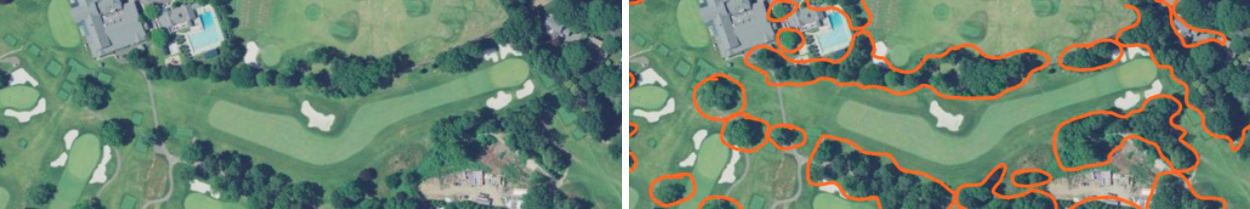
Viewing sample golf course images above, it becomes immediately apparent that trees mostly cover non-playable areas. Trees are darker than other golf course features such as bunkers, rough, green, fairway, etc. Initially, we thought that perhaps a simple thresholding approach would work to identify trees against the background golf course and implemented this approach in Python and OpenCV:

import cv2
import matplotlib.pyplot as plt


def compute_simple_mask(image):
  image_grayscale = cv2.cvtColor(image, cv2.COLOR_BGR2GRAY)
  return cv2.threshold(image_grayscale, 127, 255, 0)[1]


image_path = '...'  # e.g. https://notebooks.azure.com/clewolff/libraries/otsu/raw/golf1.jpg
image = cv2.imread(image_path, cv2.IMREAD_COLOR)
mask_simple = compute_simple_mask(image)


def show_mask(mask, image, title='', mask_color=(255, 0, 0)):
    display_image = image.copy()
    display_image[mask != 0] = mask_color
    plt.imshow(display_image)
    plt.title(title)
    plt.axis('off')
    plt.show()


show_mask(mask_simple, image, title='Simple grayscale thresholding')

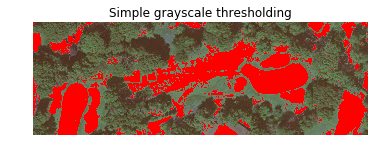
Playable area image segmentation using simple grayscale thresholding. The playable area is highlighted in red. We see that the approach does not work very well.

The image above shows all the pixels identified as “not-tree” by the algorithm as red and keeps all the “tree” pixels as their original color to provide an easy visualization to evaluate the quality of the segmentation. This visualization approach is followed in the remainder of this article.

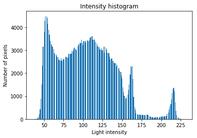
We saw that the simple thresholding approach does not work well: in addition to segmenting trees, the algorithm also segments other darker areas such as the rough. This is caused by the fact that the distribution of light intensities in the image does not have a single peak where the simple threshold can be applied.

def show_intensity_histogram(image):
    image_grayscale = cv2.cvtColor(image, cv2.COLOR_BGR2GRAY)
    plt.hist(image_grayscale.ravel(), 256)
    plt.title('Intensity histogram')
    plt.ylabel('Number of pixels')
    plt.xlabel('Light intensity')
    plt.show()


show_intensity_histogram(image)

Intensity histogram of a golf course showing a bimodal distribution leading to poor performance of simple thresholding approaches.

Otsu thresholding

To improve on the segmentation, we next investigated a smarter thresholding approach: Otsu’s method. Otsu thresholding assumes that there are two classes of pixels in the image which we wish to separate. Additionally, Otsu’s method assumes that the two classes are separated by a roughly bimodal intensity histogram. The algorithm will then find the optimal threshold that separates the two classes via an exhaustive search for the threshold that minimizes the variance between the two classes. Our golf course images seemed to fit the assumptions of the algorithm: the two classes of pixels are “trees” and “the rest” and the intuition for our bimodal intensity histogram is “trees are dark”, “the rest is light”.

def compute_otsu_mask(image):
  image_grayscale = cv2.cvtColor(image, cv2.COLOR_BGR2GRAY)
  return cv2.threshold(image_grayscale, 0, 255, cv2.THRESH_BINARY + cv2.THRESH_OTSU)[1]


mask_otsu = compute_otsu_mask(image)
show_mask(mask_otsu, image, title='Otsu grayscale thresholding')

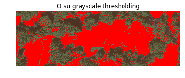
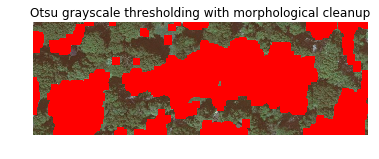
Playable area image segmentation (in red) using Otsu’s method. The mask is much better than the previous simple thresholding approach.

Using Otsu’s method for thresholding worked much better than the simple thresholding: large parts of the playable rough are now included in the segmented mask. There are some small false-positives such as the masked pixels in the tree crowns on the right upper side of the image. However, those small areas of noise were easily fixed via morphological operations such as opening, erosion and dilation.

import numpy as np

kernel = np.ones((5, 5), np.uint8)

mask_otsu_clean = cv2.morphologyEx(mask_otsu, cv2.MORPH_OPEN, kernel, iterations=2)
mask_otsu_clean = cv2.erode(mask_otsu_clean, kernel, iterations=2)
mask_otsu_clean = cv2.dilate(mask_otsu_clean, kernel, iterations=5)

show_mask(mask_otsu_clean, image, title='Otsu grayscale thresholding with morphological cleanup')

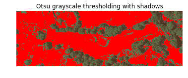
Playable area image segmentation (in red) using Otsu’s method with morphological operations to clean up noise.

One area where we noted that Otsu’s method broke down is in an image that contains shadows such as the example below. Otsu’s method operates on grayscale images so it can’t distinguish the deep dark green color of the tree canopy from the dark shadows of a tree. This is very visible in the upper center of the picture where shadows on the right end of the horizontal tree line are being included. However, for our golf course image segmentation, these shadows should be excluded.

Playable area image segmentation (in red) using Otsu’s method failing due to shadows in the image. Refer to the top center shadows on the right end of the trees.

Otsu thresholding in HLS and Lab colorspaces

One of the main limitations for Otsu thresholding as described in the previous sections is that the algorithm operates entirely on image intensity, i.e., on a grayscale image. This means that all color information is discarded. However, intuitively, for the use-case of detecting trees from the background golf course, color information should be beneficial since trees, their shadows, the fairway, rough, bunkers, etc. all have fairly distinct colors.

To better leverage color information, we converted the images into the hue-lightness-saturation (HLS) colorspace or the Lab colorspace. The HLS colorspace maps a color image from the three-dimensional RGB space into a new space with three dimensions:

The first dimension, Hue, represents the raw color, e.g. red versus green.
The second dimension, Lightness, represents the color intensity, e.g. dark versus light.
The third dimension, Saturation, represents the color fullness, e.g. washed-out versus vibrant.

Compared to RGB, the setup of the three dimensions in the HLS colorspace makes it much easier to distinguish between features in images. For example, all dark tones such as shadows will necessarily have a low lightness value in HLS colorspace; but in RGB colorspace the same pixels could have very distinct values since there are many combinations of red-green-blue values that produce a dark tone. In essence, the HLS colorspace distinguishes dimensions between chroma (color) and luma (light). The Lab colorspace is similar to HLS but uses two dimensions (a and b) to represent chroma.

def compute_otsu_mask_hue(image):
    image_hls = cv2.cvtColor(image, cv2.COLOR_BGR2HLS)

    hue, lightness, saturation = np.split(image_hls, 3, axis=2)

    hue = hue.reshape((hue.shape[0], hue.shape[1]))

    otsu = cv2.threshold(hue, 0, 255, cv2.THRESH_BINARY + cv2.THRESH_OTSU)[1]
    otsu_mask = otsu != 255

    return otsu_mask


mask_otsu_hue = compute_otsu_mask_hue(image)
show_mask(mask_otsu_hue, image, title='Otsu thresholding on the hue channel')

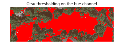
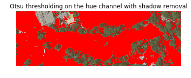
Playable area image segmentation (in red) using Otsu’s method in hue colorspace. The produced mask is much more robust than the previous grayscale approach.

We immediately saw that Otsu thresholding in HLS colorspace is a lot more robust than the previous grayscale approaches. Additionally, the HLS and L*a*b colorspaces let us perform cleanup operations to remove shadows, such as removing the darkest pixels from Otsu’s mask, which finally led us to a pre-labeling algorithm that was very usable for our golf course images:

def compute_otsu_mask_shadows(image, shadow_percentile=5):
    image_hls = cv2.cvtColor(image, cv2.COLOR_BGR2HLS)

    hue, lightness, saturation = np.split(image_hls, 3, axis=2)
    hue = hue.reshape((hue.shape[0], hue.shape[1]))

    otsu = cv2.threshold(hue, 0, 255, cv2.THRESH_BINARY + cv2.THRESH_OTSU)[1]
    otsu_mask = otsu != 255

    image_lab = cv2.cvtColor(image_2, cv2.COLOR_BGR2LAB)
    l, a, b = np.split(image_lab, 3, axis=2)
    l = l.reshape((l.shape[0], l.shape[1]))

    shadow_threshold = np.percentile(l.ravel(), q=shadow_percentile)
    shadows_mask = l < shadow_threshold

    mask = otsu_mask ^ shadows_mask

    return mask


image_path2 = '...'  # e.g. https://notebooks.azure.com/clewolff/libraries/otsu/raw/golf2.jpg
image2 = cv2.imread(image_path2)
mask_otsu_shadows = compute_otsu_mask_shadows(image2)
show_mask(mask_otsu_shadows, image2, title='Otsu thresholding on the hue channel with shadow removal')

Playable area image segmentation (in red) using Otsu’s method in hue colorspace and shadow removal in L*a*b colorspace.

Alternative approaches

As discussed in the introduction, the standard approach to create labeled datasets for image segmentation tasks is to annotate regions of interest in a collection of images manually. Even for small datasets, this approach is tedious and error-prone.

The techniques outlined in this article enable a new workflow for generating labeled data for image segmentation tasks: formulate some smart thresholding approaches, run all of them over the corpus of training images, and then have a human annotator quickly distinguish between good masks and bad masks. These approaches are somewhat ad-hoc and not extremely robust, and will therefore only work for a fraction of images in any given corpus. However, the masks can be quickly generated and it’s much more efficient for a human annotator to verify whether a mask is of high or low quality than to manually annotate regions of interest in an image. Even if only 10% of masks pass the quality control, this will still lead to a large corpus of annotated images for the training of a deep learning image segmentation model.

To further improve on the pre-labelings generated by Otsu’s method, more advanced algorithms could be explored. Idder and Laachfoubi for example showed that multi-level thresholding can outperform Otsu’s method when segmenting satellite images of clouds. As the corpus of verified labeled images grows, semi-supervised techniques such as “Learning to Segment Everything” by Hu et al can be leveraged to refine the auto-generated masks further.

Conclusion

We’ve shown how to use simple computer vision techniques like colorspace transformations and smart thresholding to automatically generate masks to train deep learning image segmentation models. A human annotator can then quickly verify these masks to create a large corpus of labeled images for model training.

To facilitate the mask generation-and-verification workflow, we’ve released image-segmentation-auto-labels, a dockerized Python application. This application can be run as a web service or command-line tool to quickly generate candidate masks for images based on a variety of segmentation approaches. Try it out and contribute your favorite masking approaches back via a pull request! You can also experiment with all the techniques outlined above in the companion Azure Notebook for this article.