Satellite Images Segmentation and Sustainable Farming

Olga Liakhovich

Introduction

Sustainability in agriculture is crucial to safeguard natural resources and ensure a healthy planet for future generations. To assist farmers, ranchers, and forest landowners in the adoption and implementation of sustainable farming practices, organizations like the NRCS (Natural Resources Conservation Services) provide technical and financial assistance, as well as conservation planning for landowners making conservation improvements to their land.

Central to efforts in sustainable farming is the process of map labeling. This process entails reviewing satellite images to determine how farmers are implementing sustainable practices. The task involves recognizing and marking visible evidence of practices such as the presence of filter strips and riparian buffers – i.e., vegetated tracts and strips of land utilized to protect water sources. Creating and maintaining a comprehensive map of sustainability practices enables experts to monitor conservation efforts over time, while also helping to identify areas that need special attention and follow-up.

However, such map labeling today still requires a manual and tedious task that teams in NRCS have to tackle daily analyzing a complex array of geospatial data sources. To perform appropriate labeling of filter strips and riparian buffers, for example, conservation specialists must closely examine images of fields and water sources, determining whether the width and border appear consistent with markings of such vegetated land conservation techniques.

To help in this effort, Microsoft partnered with Land O’Lakes SUSTAIN, which collaborates with farmers to help them improve sustainability outcomes using the latest best practices, including those recommended by NRCS.  Together, we explored ways of automating these map labeling tasks. In particular we focused our efforts on labeling waterways, terraces, water and sediment control basins, and field borders.

Our aim was to use a Unet-based segmentation model and a Mask RCNN-based instance segmentation model machine learning approaches to find a solution.  In this blog post we’ll provide details on how we prepared data, trained these models and compared their performance.  Our findings, we hope, will improve efficiency for all conservation specialists engaged in map-labeling techniques using satellite imagery analysis. The corresponding code can be found in this GitHub repo.

Data

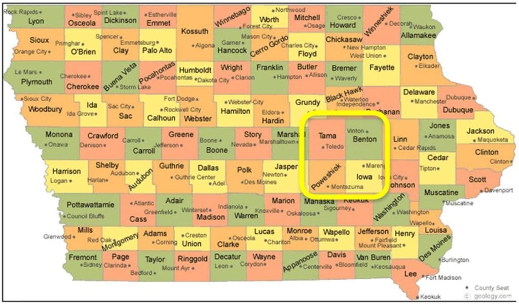
We used GeoSys satellite imagery for the following 4 Iowa counties: Tama, Benton, Iowa, and Poweshiek.

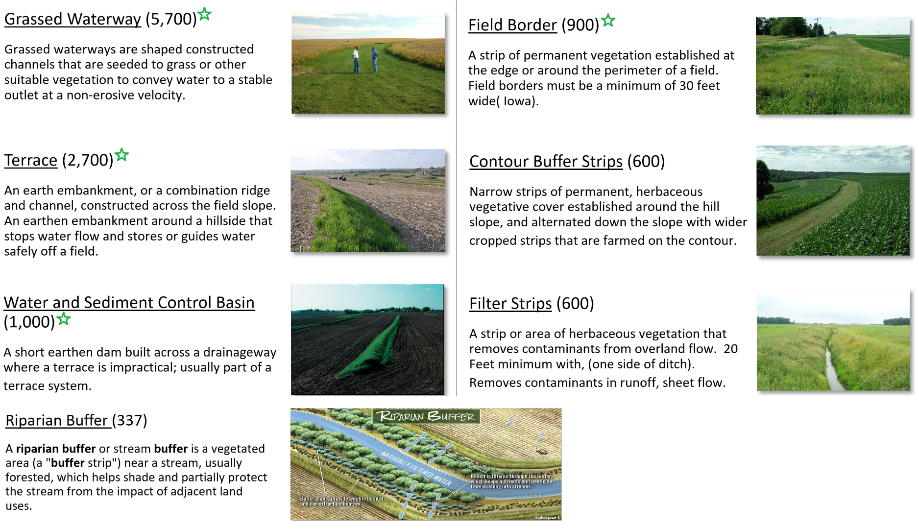
To get the training dataset, the aerial imagery was labeled manually using a desktop ArcGIS tool. The images then were split into tiles of 224×224 pixel size. Our goal was for each class to have at least 1000 corresponding tiles. The data for 7 suitable practices were prepared (see the description below). For the development of the proof of concept (POC) machine learning model we focused on the 4 classes that have the most labeled data:

• Grassed waterways (5.7K manually labeled tiles)
• Terraces (2.7K tiles)
• Water and Sediment Control Basins or WSBs (1K tiles)
• Field Borders (1K tiles).

Here is what the training data looked like:

• image tiles of 224×224 pixels size
• corresponding labels (masks) providing an outline of the region of interest.

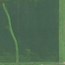
The goal was to train a model able to detect the outlines of the farming land use and correctly classify those practices.  For example, in the image below we wanted to detect waterways and counter buffer strips:

Here is a sample small dataset: it has 10 labeled images per class and gives a sense of the data we were using.

Data preparation

We augmented the dataset by flipping the image and rotating by 90 degrees. For training we used 70% of the data and 30% was saved for model evaluation.

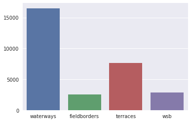
The diagram below shows the overall data distribution across classes:

After manual examination of the tiles we noticed that even for a human it’s not always possible to distinguish the land use types just by looking at an aerial image.

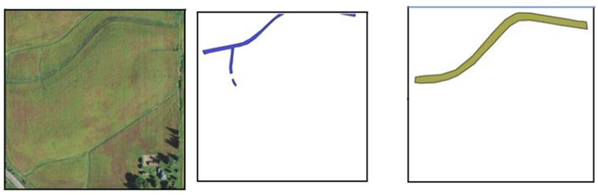
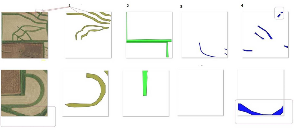
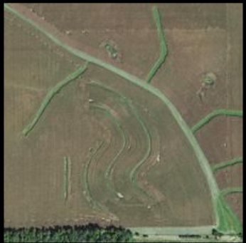
The example below highlights the challenge.  On the left we have input tiles,  followed by masks for sustainability classes that a human expert has identified on this input image. Each sustainability class has different color coding (shades of green for class 1 and 2 versus blue masks for class 3 and 4).  If we look at the first example, it appears that the top half of the image depicts a single sustainability practice. However, in reality those are different. There is a similar challenge with the second example: The central green arch belongs to class 1, but is easily confused with the lower arch which belongs to class 4.

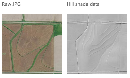
NRCS Experts heavily use DEM (hill shade data) when analyzing sustainability practices. For example, a terrace is a combination of a ridge and a channel. Contour buffer strips go around the hill slope.

So, we added hill shade data to the dataset and applied the same data augmentation techniques to it as well.

Model training infrastructure

We used Keras with a Tensorflow backend to train and evaluate models.

When training Deep Learning models it’s convenient to use hardware with GPUs.  Provisioning on demand Azure Deep Learning Virtual Machine or Azure N-series Virtual Machines  proved to be very useful.

Method

To evaluate the feasibility of identifying and classifying sustainable farming practices we took 2 approaches (as the most promising):

• Unet based segmentation model
• Mask RCNN based instance segmentation model

Introduction to Unet

U-Net is designed like an auto-encoder. It has an encoding path (“contracting”) paired with a decoding path (“expanding”) which gives it the “U” shape.

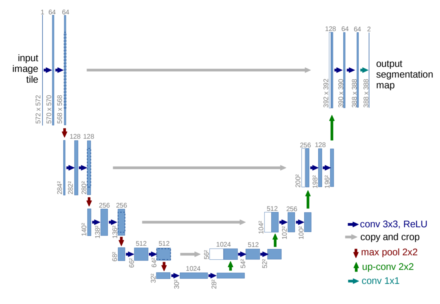
However, in contrast to the autoencoder, U-Net predicts a pixelwise segmentation map of the input image rather than classifying the input image as a whole. For each pixel in the original image, it asks the question: “To which class does this pixel belong?”. U-Net passes the feature maps from each level of the contracting path over to the analogous level in the expanding path.  These are similar to residual connections in a ResNet type model, and allow the classifier to consider features at various scales and complexities to make its decision.

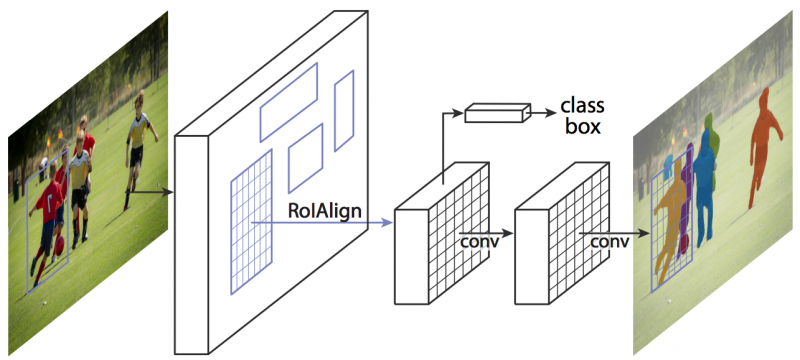
Introduction to Mask RCNN

Mask RCNN (Mask Region-based CNN) is an extension to Faster R-CNN that adds a branch for predicting an object mask in parallel with the existing branch for object detection. This blog post by Dhruv Parthasarathy contains a nice overview of the evolution of image segmentation approaches, while this blog by Waleed Abdulla explains Mask RCNN well.

Metrics and loss functions

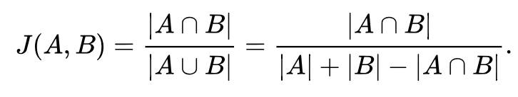
Our primary metric for model evaluation was Jaccard Index and Dice Similarity Coefficient. These both measure how close the predicted mask is to the manually marked masks, ranging from 0 (no overlap) to 1 (complete congruence).

Jaccard Similarity Index is the most intuitive ratio between the intersection and union:

Dice Coefficient is a popular metric and it’s numerically less sensitive to mismatch when there is a reasonably strong overlap:

Regarding loss functions, we started out with using classical Binary Cross Entropy (BCE), which is available as a prebuilt loss function in Keras.

Inspired by this repo related to Kaggle’s Carvana challenge, we explored incorporating the Dice Similarity Coefficient into a loss function:

Training Segmentation Model

Below we describe the training routine using Mask RCNN and Unet and discuss our learnings.

Training with Unet

When dealing with segmentation-related problems, Unet-based approaches are applied quite often – good examples include segmentation-themed Kaggle competitions (e.g., DSTL satellite imagery feature detection, Carvana car segmentation), as well as various medical-related segmentation tasks (e.g., segmenting nerves in ultrasound images, lungs in CT scans, and robotics instrument segmentation for endoscopy).

Two of the benefits of Unet are that:

• It can be trained on a modestly-sized dataset
• Its input can easily be converted from 3 channels (standard RGB image) to more interesting inputs as multispectral images

Training a Unet model on 2 classes (waterways and field borders) with 600 training images for 25 epocs produced promising results right away.

Note: In machine-learning parlance, an epoch is a complete pass through a given dataset.

Input image:

Below are the prediction results for a simple 2-class model trained from scratch on just a few hundred tiles:

Here we can see that the label is not perfect in the image: there is a field border on the right and something that looks very similar to a field border at the bottom (though the bottom instance is not labeled). The model detects both right and bottom borders.

Using hill shade data

As mentioned earlier, DEM info is very handy when detecting sustainable images. We converted hill shade data to a grayscale image and added this info as an additional 4th input channel.

Pre-initializing weights for Unet

In the above example we’re training Unet “from scratch” on our data.  However smart weights initialization usually saves training time and positively affects the results (see TernausNet for more details on how U-Net type architecture can be improved by the use of the pre-trained encoder).

We trained Unet on 4 channel input: 3 channels were used for RGB input and the 4th channel was used for hill shade data.  Weights for the first 3 channels are initialized from VGG 16 model pre-trained on the ImageNet dataset. We were leaving the 4th channel initialized with zeroes — further improvements might include experimentation with various weights initialization techniques. See model.py for more details.

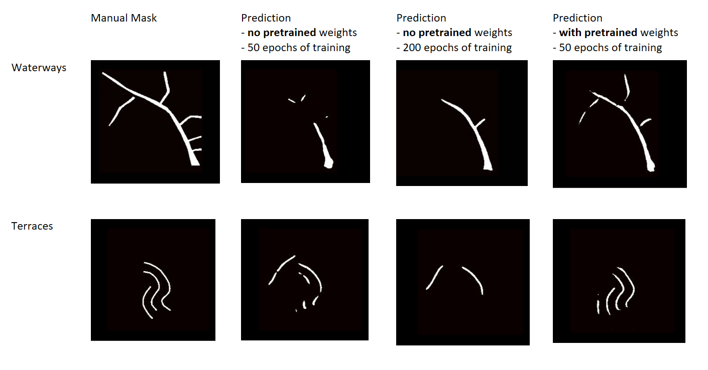
Below are visual comparisons of the results: manual label (left), training Unet from scratch (middle), training Unet with leveraging VGG16 weights pre-trained on ImageNet (right).

Input raw image:

Results: as expected, the Unet model that uses pre-trained VGG16 can learn much faster.

Training with Mask-RCNN

In general, a significant number of labeled images are required to train a deep learning model from scratch.  We experimented with training a MaskRCNN model from scratch and the results were not promising at all after 48 hours of training (1 Titan Xp GPU).

To overcome the challenge and save training time we again used transfer learning. We re-used the Mask RCNN model pre-trained on the COCO dataset, then fine-tuned the model on the dataset with aerial images.

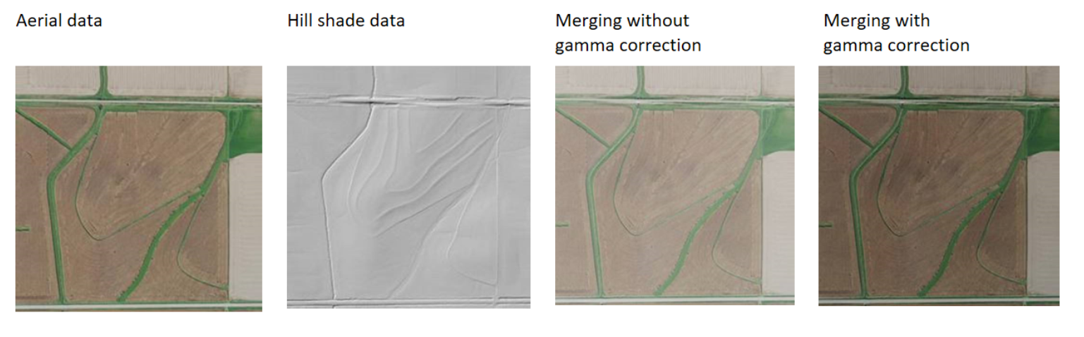
As we discussed in the Data Preparation section, hill shade data is very useful for detecting some of the classes (terraces for example). So, ideally, we wanted to have a means to provide training input in at least 4 channels: 3 channels for RGB aerial photos and 1 more channel for hill shade data. The issue we encountered was that current pre-trained models work well only with 3 channel input. Thus we merged the RGB and hill shade tiles into a combined 3 channel tile and used the later for training. We noticed that using gamma correction on the merged images improves the results: the image with gamma correction is less “bleached out,” while vegetation and topographical features are more prominent.

Below we demonstrate the MASK RCNN model prediction results and how they vary depending on whether or not the model had access to hill shade data and the loss function: the original input is most left, then there is the prediction result for the model trained only on aerial data. Following are prediction results for the model that was trained on a combination of aerial and hill shade data. Finally we show results for a model trained on a combination of aerial and hill shade data, using the enhanced loss function (takes Dice Coefficient into consideration).

As identification of terraces relies mainly on hill shade information, the mask prediction tended to work better if the model was trained on data that also had information about the area’s topography. Incorporating Dice Coefficient seemed to add positive improvements as well.

In the next diagram we show how the Mask RCNN models prediction evolved as the model trained for a longer time (more epochs). For demonstration we’re using the same cherry-picked example that we used in Unet’s section of this blog (see Pre-initializing weights for Unet) . In this example we’re using a model trained on aerial and hill shade data and a loss function that uses Dice Coefficient:

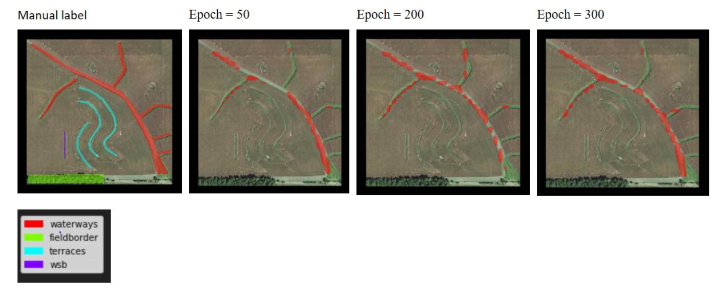
It is worth noting how distinct “instances” of waterways merge as training progresses: at the beginning (epoch 50) most of the waterway predictions are separate pieces and the center part of the waterway is absent from the prediction. However, beginning at Epoch 200, the predicted mask covers more and more surface and gets much closer to the manual label.

As a side note, the Mask RCNN was not able to detect terraces in this example, while the Unet model did find terraces.

Results

Both the Mask RCNN and the Unet models did a fairly good job of learning how to detect waterways – this was no surprise, as this class has the biggest amount of labeled data. The average Dice Coefficient (on test set, around 3000 examples) for the Mask RCNN and the Unet models for waterways was 0.6515 and 0.5676, respectively.

The histogram below shows the distribution of Dice Coefficient values for waterways across the test set for Mask RCNN and Unet:

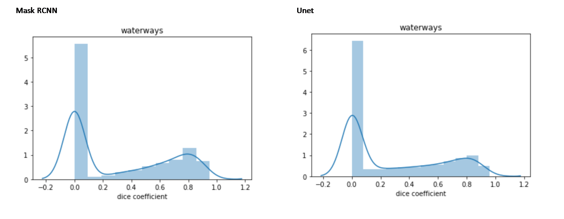
Our tests showed that the mean Dice Coefficient across all classes is a bit higher for the Mask RCNN model. Incorporating the Dice Coefficient had a positive impact on the Mask RCNN model performance. For Unet models, it improves performance in detecting waterways, but there is no significant difference for other classes.

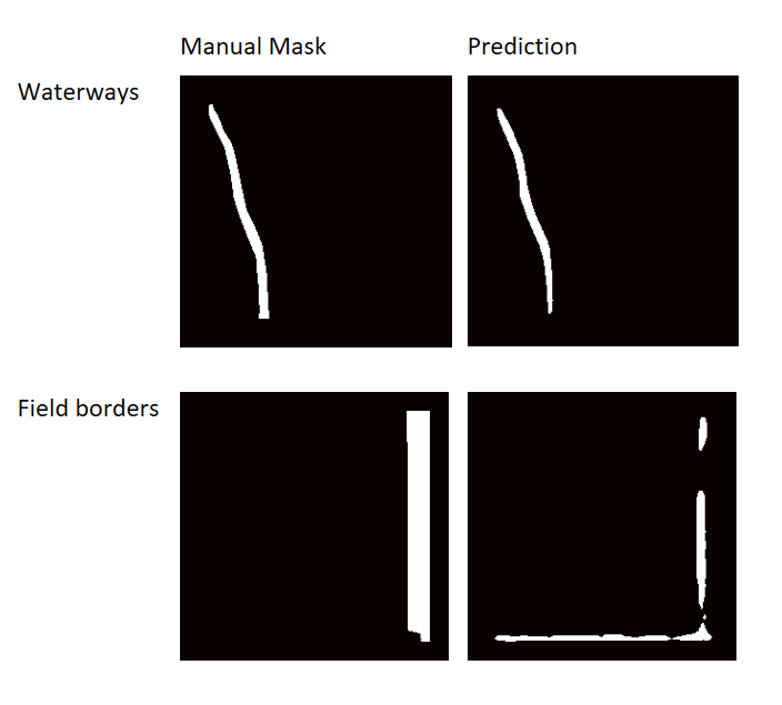
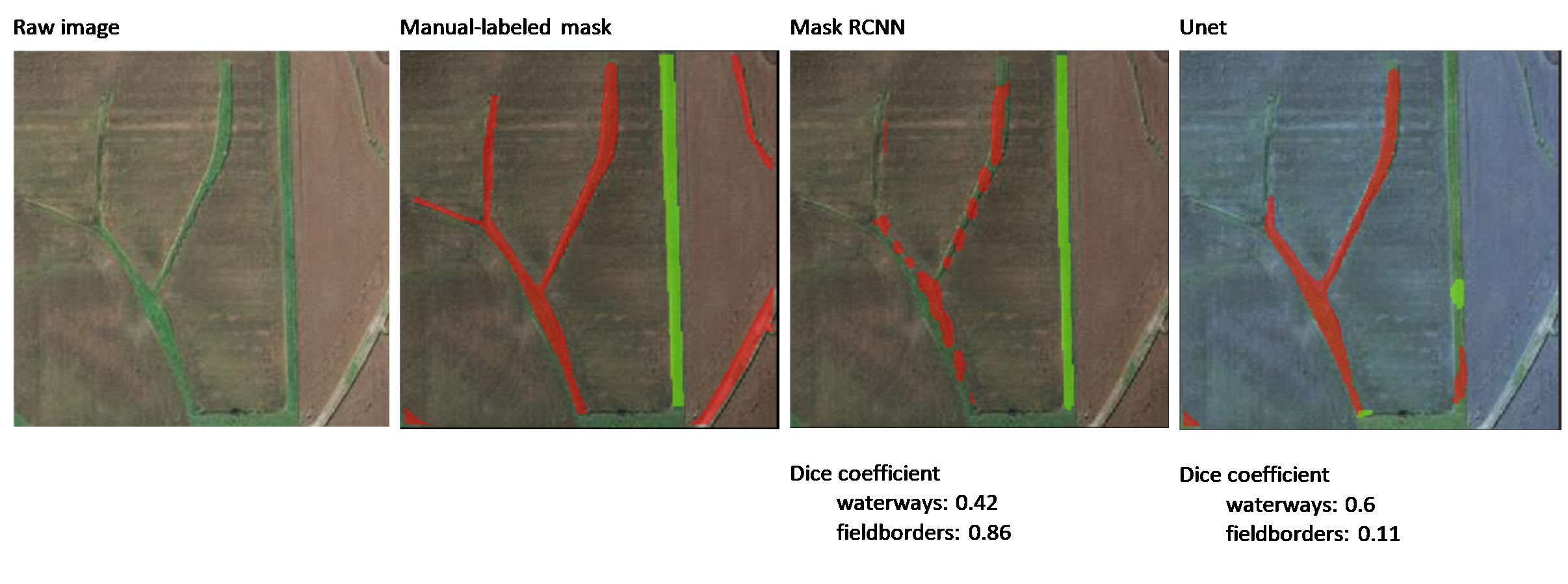
We used the mean Dice Coefficient to select the best Mask RCNN model. It was trained on a combination of aerial and hill shade data, using the enhanced loss function. The images below show a visual comparison of the Mask RCNN and Unet model predictions on a cherry-picked example. As we can see, both the Mask RCNN and Unet models performed decently in detecting waterways. Although the dice value of waterways is not very large (0.42), the model is definitely on the right track to detect waterways. The Mask RCNN detection of field borders almost covers the manual-labeled mask, which is very impressive. However, the Unet model only starts picking up the field border.

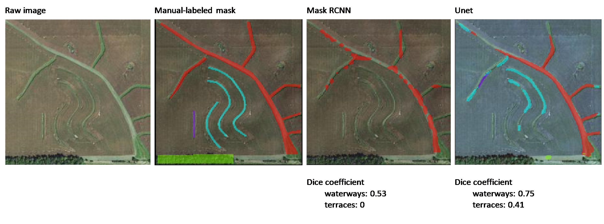
Below is another example demonstrating the results of the terrace’s detection. In this example, the Mask RCNN does not detect the terraces and the Unet does (hopefully making good use of hill shade data). Although the Dice Coefficient value of terraces is not very large (0.41), the prediction already captures the main shape of terraces and thus is useful for practical applications.

Incorporating additional channels of information such as hill shade data or multi band satellite imagery is definitely a promising approach. Doing so with Unet seems to be more straightforward than with Mask RCNN.

Conclusions and Discussion

We saw really promising results with getting AI to help with the detection of sustainable farming practices. Future work may include enhancing the dataset and making it more balanced, as well as getting additional channels of information (multispectral and hyperspectral images) and exploring performance with specialized models that detect only 1-2 classes.

In addition to this work’s potential applications for sustainable farming, similar work could be utilized in detecting solar panels or green-garden roofs in smart eco-friendly cities.

References

1. Github repo.
2. “Mask RCNN” paper.
3. “U-Net: Convolutional Networks for Biomedical Image Segmentation” paper.
4. Mask RCNN Keras implementation github repo.
5. “TernausNhttps://github.com/matterport/Mask_RCNNet: U-Net with VGG11 Encoder Pre-Trained on ImageNet for Image Segmentation” paper
6. Carvana Image Masking Kaggle challenge 4th place winners repo.

Featured photo by Sveta Fedarava on Unsplash

Olga Liakhovich

Follow