Learning Image to Image Translation with Generative Adversarial Networks

We recently worked with our partner Getty Images, a global stock photo agency, to explore image to image translation on their massive collection of photos and art. The ability to use Deep Learning to change the aesthetics of a stock image closer to what the customer is looking for could be game-changing for the industry. With recent advancements in Generative Adversarial Networks (GANs), specifically PIX2PIX image mapping and CycleGANs, such image translation is now possible.

Background

While Deep Convolutional Networks have greatly improved the ability for computers to see and understand images in recent years, the ability to generate or manipulate images into a different visual space was still prohibitively difficult. A significant breakthrough occurred, however, with the development of Generative Adversarial Networks (GANs). Yann LeCun, one of the fathers of Deep

Learning, has described GANs as the most important idea in Machine Learning in the last 20 years.

For this project, we’ve focused on the application of GANs in image-related tasks, but it is worth mentioning that they are not limited to them (for example, this text application of GANs).

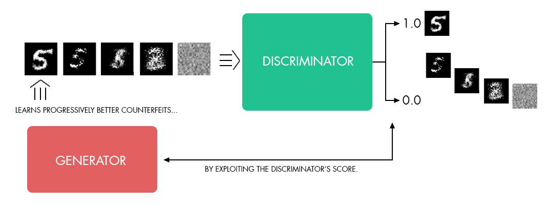
The core idea behind a Generative Adversarial Network is to create two models and have them compete against each other in order to improve them both through competition. The first model can be considered a discriminator, which is trained to recognize a particular type of image. For example, a discriminator can be taught to recognize images of handwritten digits with training on the classic MNIST dataset. The discriminator’s goal is to accurately score any incoming images as either “Yes, this looks like a handwritten digit from the training dataset” or “No, this is not an image of a handwritten digit” for any other type of image.

Image 01 discriminator

The other party in this adversarial “wrestling” game is our generator — a model capable of counterfeiting images. The generator competes against this discriminator and generator’s sole task is to learn to create synthetic images that will eventually be good enough to fool the discriminator. The generator uses the discriminator’s score as its feedback mechanism for improving itself over time (and thus make images look more “realistic”).

Image 02 disc gen

Once the power of GANs started to be understood and applied, machine learning experts began creating even more powerful solutions by fighting teams of GANs against each other. This method allows us to generate a certain type of image artificially, such as the handwritten digits in the example above. It also allows us to have a pair of discriminators that have learned two related types of images compete against a pair of generators working to fool them so that the GAN would learn how to manipulate images from one type into its counterpart type. We call this image-to-image translation.

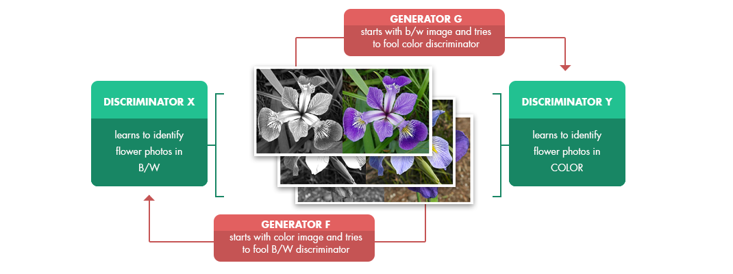
Image 03 pix 2 pix 1

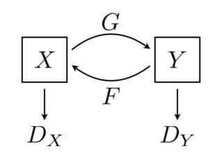
For example, if you have training data that presents two copies of a photo of a flower, one in black and white and the other copy in color, you can set up a discriminator for each side. One discriminator will learn to identify the black and white aesthetic, while the other one will learn to recognize color photos. The generators do not attempt to fool their target discriminators from scratch; instead, they begin by using an image from the opposite collection. In this example, Generator G attempts to fool the Color Discriminator Y by starting with a black and white photo and then manipulating it until it is colored successfully. Similarly, Generator F starts with a color image and learns how to desaturate it well enough to fool the black and white discriminator.

Once this model architecture is properly trained, the GAN allows us to translate an image from one aesthetic profile to another. We can then take one type of picture and convert it to another, as long as our GAN has been properly trained on both types of images.

This model was popularized with the famous PIX2PIX paper. A fantastic write up on PIX2PIX and how the generators and discriminators work at a lower level can be found in this article.

CycleGANs

While PIX2PIX can produce truly magical results, the challenge is in training data. The two image spaces that you wanted to learn to translate between needed to be pre-formatted into a single X/Y image that held both tightly-correlated images. This could be time-consuming, infeasible, or even impossible based on what two image types you were trying to translate between (for instance, if you didn’t have one-to-one matches between the two image profiles). This is where the CycleGAN comes in.

The key idea behind CycleGANs is that they can build upon the power of the PIX2PIX architecture, but allow you to point the model at two discrete, unpaired collections of images. For example, one collection of images, Group X, would be full of sunny beach photos while Group Y would be a collection of overcast beach photos. The CycleGAN model can learn to translate the images between these two aesthetics without the need to merge tightly correlated matches together into a single X/Y training image.

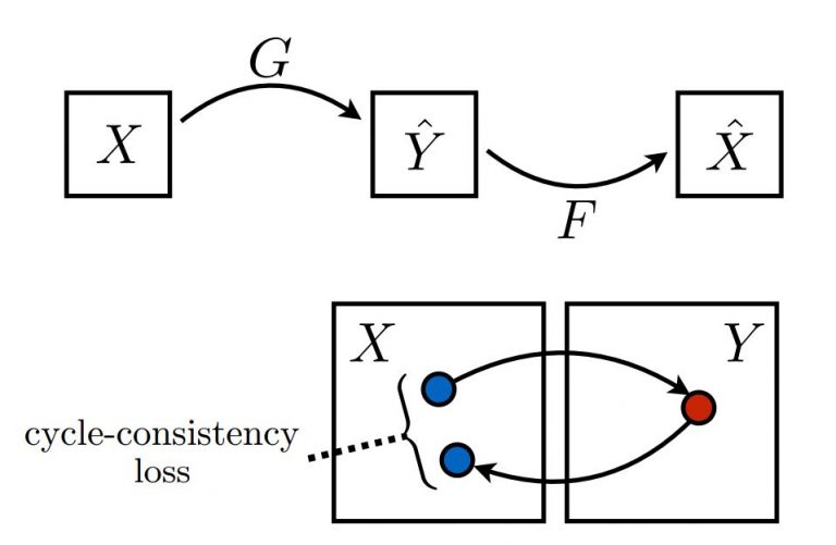
The way CycleGANs are able to learn such great translations without having explicit X/Y training images involves introducing the idea of a full translation cycle to determine how good the entire translation system is, thus improving both generators at the same time.

Image full cycle 768 215 501

For example, if you have an English phrase and use an online English-to-Spanish translation system to translate the phrase into Spanish, you will get one result. When you then take that translated result and re-translate it through the complementary Spanish-to-English translator, you will now have a full cycle of translation. Comparing how similar the resulting English-Spanish-English translated phrase is to the original English input gives you an additional score that you can use to improve your entire translation system. This approach is the clever power that CycleGANs brings to image-to-image translations and how it enables better translations among non-paired image styles.

The original CycleGANs paper, “Unpaired Image-to-Image Translation using Cycle-Consistent Adversarial Networks”, was published by Jun-Yan Zhu, et al. The accompanying code was written in Torch and hosted on GitHub. However, for our Getty Images hackfest, we decided to implement a CycleGAN in TensorFlow which can be trained and hosted on Azure. We chose TensorFlow because there were existing CycleGAN implementations we could draw from. We also felt TensorBoard would help us visualize the complexity of the CycleGAN architecture. In addition, we had expertise in distributed training using Kubernetes and with the strict time-frame of a hackfest, we needed all the help we could get. Later we were able to focus on migrating the code to the Microsoft Cognitive Toolkit (see project repo).

For our training images, we decided to take advantage of the treasure trove of stock photos Getty Images maintains and created four different image groups over two different CycleGAN models. One CycleGAN model would learn to translate sunny beach photos to overcast beach photos while a second CycleGAN would learn to translate between daytime and sunset beach photos.

The Code

Our TensorFlow implementation of CycleGANs can be found on GitHub.

Input Pipeline

The first step in training GANs is to load images. We use tfrecord format for a more effective image loading pipeline comparing to one-by-one image loading from disc. We assume that your images for CycleGANs training and testing are in the following folders:

trainA: train images for the class A (for example, sunny beach)
trainB: train images for the class B (for example, cloudy beach)
testA: class A test images
testB: class B test images

Run to_tfrecords.py to convert images in the directories above to a corresponding binary representation in tfrecord format. During training, images will be loaded in batches from tfrecords files using the Images class defined in image.py.

 real_X = Images(args.input_prefix + '_trainA.tfrecords', batch_size=BATCH_SIZE, name='real_X').feed()
 real_Y = Images(args.input_prefix + '_trainB.tfrecords', batch_size=BATCH_SIZE, name='real_Y').feed()

Generator and discriminator

In this section, we will go more into implementation details depth assuming the reader has some familiarity with how to build CNNs in TensorFlow.

The training graph and main training routines are defined in cyclegan.py (for network architecture details refer to the original paper by Jun-Yan Zhu). The generator is defined in the “generator” function:

def generator(image, norm='batch', rnorm='instance', reuse=False, name="generator")

The generator consists of the blocks mentioned in the original paper:

This network contains two stride-2 convolutions, several residual blocks [14], and two fractionally-strided convolutions with stride 1 2 .

In addition, we’re extended this architecture with few touch ups from the paper Perceptual Losses for Real-Time Style Transfer and Super-Resolution.

All nonresidual convolutional layers are followed by batch normalization and ReLU nonlinearities with the exception of the output layer, which instead uses a scaled tanh to ensure that the output has pixels in the range [0, 255].

Here is how this network architecture could be defined via the TensorFlow APIs:

 # define stride-2 convolutions 
 s = 256
 c = tf.pad(image, [[0, 0], [3, 3], [3, 3], [0, 0]], "REFLECT")
 c = tf.nn.relu(do_norm(conv2d(c, 32, 7, 1, padding='VALID', name='g_e1_c', reuse=reuse), norm, name + 'g_e1', reuse))
 c2 = tf.nn.relu(do_norm(conv2d(c, 64, 3, 2, name='g_e2_c', reuse=reuse), norm, 'g_e2', reuse))
 c3 = tf.nn.relu(do_norm(conv2d(c2, 128, 3, 2, name='g_e3_c', reuse=reuse), norm, 'g_e3', reuse))
 # define 9 resnet blocks
 r1 = residual_block(c3, 128, norm=rnorm, name='g_r1', reuse=reuse)
 r2 = residual_block(r1, 128, norm=rnorm, name='g_r2', reuse=reuse)
 ...
 r9 = residual_block(r8, 128, norm=rnorm, name='g_r9', reuse=reuse)
 # deconvoutions to size up the image back
 d1 = deconv2d(r9, 64, 3, 2, name='g_d1_dc', reuse=reuse)
 d1 = tf.nn.relu(do_norm(d1, norm, 'g_d1', reuse))
 d2 = deconv2d(d1, 32, 3, 2, name='g_d2_dc', reuse=reuse)
 d2 = tf.nn.relu(do_norm(d2, norm, 'g_d2', reuse))
 d2 = tf.pad(d2, [[0, 0], [3, 3], [3, 3], [0, 0]], "REFLECT")

 # output layer with scaled tanh
 pred = conv2d(d2, 3, 7, 1, padding='VALID', name='g_pred_c', reuse=reuse)
 pred = tf.nn.tanh(do_norm(pred, norm, 'g_pred', reuse))

As recommended by the CycleGAN authors, instance normalization should be used in residual blocks and we noticed that indeed does improve quality. The discriminator part of the graph has consequentially similar architecture (though different convolutions, filters, and strides numbers). The output of the discriminator is a “decision” whether the given image is fake (produced by the generator) or from the real dataset.

Loss functions

The power of CycleGANs is in how they set up the loss function, and use the full cycle loss as an additional optimization target.

As a refresher: we’re dealing with 2 generators and 2 discriminators.

Generator Loss

Let’s start with the generator’s loss functions, which consist of 2 parts.

Part 1:

The generator is successful if fake (generated) images are so good that discriminator can not distinguish those from real images. In other words, the discriminator’s output for fake images should be as close to 1 as possible. In TensorFlow terms, the generator would like to minimize:

 g_loss_G_disc = tf.reduce_mean((discY_fake - tf.ones_like(discY_fake)) ** 2) 
 g_loss_F_dicr = tf.reduce_mean((discX_fake - tf.ones_like(discX_fake)) ** 2)

Note: the “**” symbol above is the power operator in Python.

Part 2:

We need to capture cyclic loss: as we go from one generator back to the original space of images using another generator, the difference between the original image (where we started the cycle) and the cyclic image should be minimized.

g_loss_G_cycle = tf.reduce_mean(tf.abs(real_X - genF_back)) 
               + tf.reduce_mean(tf.abs(real_Y - genG_back))
g_loss_F_cycle = tf.reduce_mean(tf.abs(real_X - genF_back)) 
               + tf.reduce_mean(tf.abs(real_Y - genG_back))

Note: the “” symbol in this context (Python) means that statement spans several lines.

Finally, the generator loss is the sum of these two terms:

g_loss_G = g_loss_G_disc + g_loss_G_cycle

Because cyclic loss is so important we want to multiply its effect. You can make a comparison to measuring the quality of a translator: if you translate a phrase from English to Spanish, then from Spanish to English and result is close to the original, then the translator is good. Similarly, with Cycle GANs, after doing a cycle of transformation the resulting image should be close to the original.

We used an L1_lambda constant for this multiplier (in the paper the value 10 was used).

Now the grand finale of the generator loss looks like:

g_loss_G = g_loss_G_disc + L1_lambda * g_loss_G_cycle
g_loss_F = g_loss_F_disc + L1_lambda * g_loss_F_cycle

Note: in the cyclegan.py you will see generator loss defined in one statement. We also experimented with soft labels for g_loss_G_disc and g_loss_F_disc logical parts; rather than requiring a strong “Yes” (meaning 1) from the discriminator we allowed “Quite sure” (0.95 for example).

Discriminator Loss

The Discriminator has 2 decisions to make:

Real images should be marked as real (recommendation should be as close to 1 as possible)
The discriminator should be able to recognize generated images and thus predict 0 for fake images.

DY_loss_real = tf.reduce_mean((DY - tf.ones_like(DY))** 2)
DY_loss_fake = tf.reduce_mean((DY_fake_sample - tf.zeros_like(DY_fake_sample)) ** 2)
DY_loss = (DY_loss_real + DY_loss_fake) / 2

DX_loss_real = tf.reduce_mean((DX - tf.ones_like(DX)) ** 2)
DX_loss_fake = tf.reduce_mean((DX_fake_sample - tf.zeros_like(DX_fake_sample)) ** 2)
DX_loss = (DX_loss_real + DX_loss_fake) / 2

Training and Results

Building the CycleGAN model and importing data is a significant accomplishment. However, during the training phase, we needed to experiment with various hyperparameter configurations such as batch size, learning rate, and momentum. Since the purpose of this CycleGAN is to generate aesthetically appealing results, we also experimented with the training data itself. Would a higher number of lower quality images learn better than a smaller amount of more highly curated images?

To explore this question, we created a quick Python program that allowed us to load videos of beaches and capture screen grabs repeatedly to generate many training images very quickly. Here is the code:

import numpy as np
import cv2

SPEED = 25
cap = cv2.VideoCapture('./source/beach/beachvideo.mp4')

capture_run = np.random.randint(1000)
totalFrames = 0

def capture_square(frame, square_size, capture_run, totalFrames):
     startX = np.random.randint( int((w-square_size)) )
     startY = np.random.randint( int((h-square_size)) )
     capture = frame[startY:startY+square_size, startX:startX+square_size]
     cv2.imwrite("./captures/cap{0}_f{1}.jpg".format(capture_run, totalFrames), 
     capture, [int(cv2.IMWRITE_JPEG_QUALITY), 90])
     totalFrames = totalFrames+1

while(cap.isOpened()):
     ret, frame = cap.read()
     h, w, c = frame.shape
     cv2.imshow('frame', frame)

     if (h < 600) or (w < 600):
          print("width or height of video must be at least 600px")
          break

     key = cv2.waitKey(SPEED)

     # CAPTURE FRAMES WHEN SPACE IS PRESSED
     if key == 32:
          square_size = 600
          capture_square(frame, square_size, capture_run, totalFrames)
          totalFrames = totalFrames + 1

     # QUIT ON 'Q'
     if key == ord('q'):
          break

cap.release()
cv2.destroyAllWindows()

For our task, this approach didn’t deliver a better quality result than the superior images we had access to from Getty Images. However, it provides an interesting avenue for additional CycleGAN projects and we may return to it as a training data source in the future.

Once we had a stable model and good set of training data image sets, we began running various training sessions overnight leveraging both local machines and Azure VM instances to compare various runs concurrently.

During the run, we would periodically check with TensorBoard to see how well our model was doing. TensorBoard proved invaluable for monitoring our model. However, it seemed to struggle with graphing the model itself, so CycleGANs might be a bit much for it:

Graph of CycleGAN from TensorBoard

We set up TensorBoard variables that allowed us to monitor not only our loss functions, learning rate decay, and other important parameters but also provided us with glimpses into the images being generated by our model. During training these varied from bizarre to strangely beautiful before settling down to results that looked closer to our goal. Here’s an example of an exotic sunset from one of our runs:

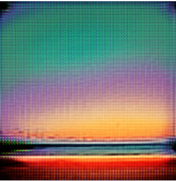
Artificial sunset

Even if we could never generate photorealistic results, we could at least generate science fiction book covers! Here is a cherry-picked sample of our results at the end of the hackfest, showing that in many cases we approached our goal.

While some of the results were very impressive, there are further optimizations we would like to explore in the future. Additional GANs can be supplemented to help clean up various artifacts created in the process, as well as to allow us to have better resolution while improving the output size. There are also traditional post-processing techniques that can be applied which don’t require deep learning and can improve the aesthetic quality and color balance of the images, which would be valuable if this approach eventually moves toward production quality.

Conclusion

Generative Adversarial Networks are at the forefront of Deep Learning research right now, and CycleGANs are one of the newest methods. We love that our team gets the chance to explore the possibilities of this new technology with partners committed to innovation. The impact of this technology on the creative sector is going to be immense, so we’re trying to ensure that we use approaches that augment creative abilities rather than replace them.

Generative Networks such as the one above are almost always shown operating in the visual realm. One reason is the Convolutional/Deconvolutional nature of the networks, but another large contributor is the striking visual impact of the resulting images. However, we see future generative networks operating in other domains (audio, text, gene sequences, etc.) to help us generate new data for training or, with guidance, creating new works. How can we design loss functions for judging the “aesthetics” of these results? Will other generator and discriminator network topologies produce better results in different domains? There are many open questions, and it’s an exciting time to be working in this field.

If you try out our code on GitHub, please let us know and share your results! If you liked this work, please share it — the more people exploring these emerging questions, the faster we’ll solve them which will benefit us all.

2 comments

Discussion is closed. Login to edit/delete existing comments.

Sort by :

Newest

Newest Popular Oldest

Andrew W. June 18, 2017 0

olga, rick and michael, have you seen any startups applying this technology to their products?
- Olga Liakhovich June 19, 2017 0
  
  These are super new technologies, CycleGans paper is literally few month old. I’ve seen some pix2pix apps, for example this one https://play.google.com/store/apps/details?id=com.dneural.drawzee&hl=en