In this post, Senior App Dev Manager Randy Park performs an exploratory data analysis using R and Azure Machine Learning Studio.
Suppose we have to design a black box which will display a “thumbs up” or “thumbs down” depending on hundreds of different combinations of inputs, we probably have a general idea of utilizing machine learning methodologies designing of the black box, here we call it a model. But often, more important question than how to build the model is rather how we can find out by looking at the proposed model, which of the input is more important than others. What is the weightiest input or feature to drive the outcome? We may think such problem is rather simple in this day and age, where abundance of machine learning algorithms and models are readily available. Once we start to analyze the each of implementation deeper and engage into coding or hands-on exercise, we come to appreciate the simple abstractions on the complexities underneath. We, however, will see outcome of design approach may not necessarily result the same outcome, and digging in details may provide further insights on the exploratory data analysis (EDA).
Objective: Put it more practically, the exercises in this article will utilize a very popular exercise dataset to conduct EDA to determine factors that lead to attrition. The snapshot of data with first 12 columns, out of 35 total columns is as below.:
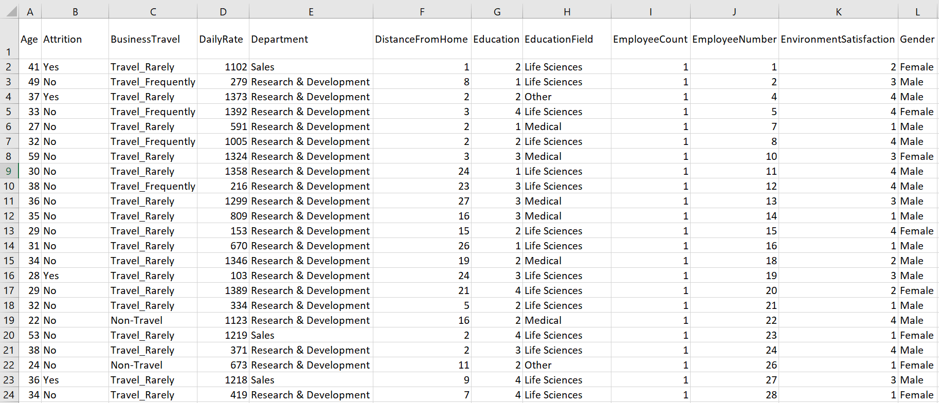
We will compare high level findings by common implementations in R vs. utilizing Machine Learning modules provided by Azure Machine Learning Studio.
R implementation using Microsoft R Client or R Studio
Using R, we will utilize simple finding of correlation coefficients to locate highest correlating coefficients with the Attrition.
We will utilize Azure machine learning studio to utilize simple and powerful permutation feature importance.
There are many implementations of above-mentioned dataset; anyone can find abundance of implementations linked to the dataset hosted in kaggle.com. Practical outcome of such exploratory data analysis is to identify at least the top three or four factors that contribute to employee turnover. Each of the analysis should be backed up by robust experimentation and where applicable, the appropriate visualization and you will find plenty examples in kaggle.com and others alike.
1. R implementations using with Microsoft R Client or R Studio
Follow installation of Microsoft R client instructions in this Microsoft R Client introduction documentation. Or you can choose to utilize popular OSS tool of R Studio.
Below steps are not necessarily the entire code and not naming all the R package requirements, rather highlights the key details of implementation in R.
1. Import Data and prepare the data frame to operate computations.
## Import the data
case_data<-data.frame(read_excel("Data/attrition-data.xlsx"))
2. Preprocess
We need to remove non value-added variables from the dataset
- EmployeeCount: Always 1, since the data set is by employee.
- Over18: All employees are “Y”. Age is a more meaningful and relevant variable.
- StandardHours: All are “80”.
## Remove redundandt info: EmployeeCount, Over18, StandardHours
df<-case_data[,-c(9,22,27)]

## Convert characters to factors
df %>% map_if(is.character, as.factor) %>% as_data_frame -> df

## Adjust factor levels as needed
levels(df$BusinessTravel)<-c("Non-Travel","Travel_Rarely","Travel_Frequently")

## Make all variable numeric
numdf<-data.frame(sapply(df,as.numeric))
3. Calculate correlation coefficients to locate highest correlating coefficients with the Attrition.
## Correlate variables
Attcor<-data.frame(cor(numdf))

## Create Attrition object for Attrition correlation coefficients
Attrition<-data.frame(Attcor$Attrition)

## Name attrition rows
Attrition$Parameter<-row.names(Attcor)

## Rename titles Attrition
names(Attrition)<-c("Correlation", "Parameter")

## Sort positive Attrition
SortAtt<-Attrition[order(-Attrition$Correlation),]

## Display top 10 Positively Correlated Parameters
row.names(SortAtt)<-NULLknitr::kable(head(SortAtt, 10))
The output of above command is as below:
| Correlation | Parameter |
|---|---|
| 1.0000000 | Attrition |
| 0.2461180 | OverTime |
| 0.1620702 | MaritalStatus |
| 0.0779236 | DistanceFromHome |
| 0.0671515 | JobRole |
| 0.0639906 | Department |
| 0.0434937 | NumCompaniesWorked |
| 0.0294533 | Gender |
| 0.0268455 | EducationField |
| 0.0151702 | MonthlyRate |
What does the above outcome highlight? Perhaps one can come to below observations:
| Top 3 Parameters | Initial Observation |
|---|---|
| Overtime | Higher reported Overtime, employees are more likely to leave |
| Marital Status | Single employees are more likely to leave. This observation may be tied to other factors and can be challenging for company to address |
| Distance from Home | Farther employees (employees whose home is farther from work) are more likely to leave |
This should not be looked as if de-facto conclusion regarding attrition, but rather one of many possible observations. As any of exploratory data analysis (EDA) leads to, the outcome is dependent upon the exploration methods, algorithm and how you prepare the data .. etc.
2. Utilizing Azure Machine Learning Studio
Before we get into the implementation specifics, it is beneficial to remind the typical five stages of machine learning implementations. Borrowing from the Microsoft Azure Machine Learning Studio Capabilities Overview diagram, below figure explains the those stages of the machine learning implementation. This approach should be also utilized in any of machine learning projects such as R, python or ML.Net.
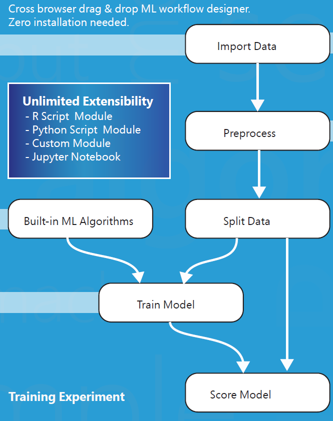
To those who are experienced in machine learnings, they would mention of two possible approaches to solve this problem. First, Filter Based Feature Selection and second, Permutation Feature Importance.
They seem to accomplish similar tasks in that both assign scores to variables so that we can identify which variables or features are significant. However, the approach of each determination is quite different. Note the definition of each from Microsoft documentation:
- Filter Based Feature Selection (FBFS) – Identifies the features in a dataset with the greatest predictive power.
- Permutation Feature Importance (PFI) – Computes the permutation feature importance scores of feature variables given a trained model and a test dataset.
We will compare each outcome to the previously hand-coded R implementation.
First, login to studio.azure.net and create a Permutation Feature Importance (PFI).
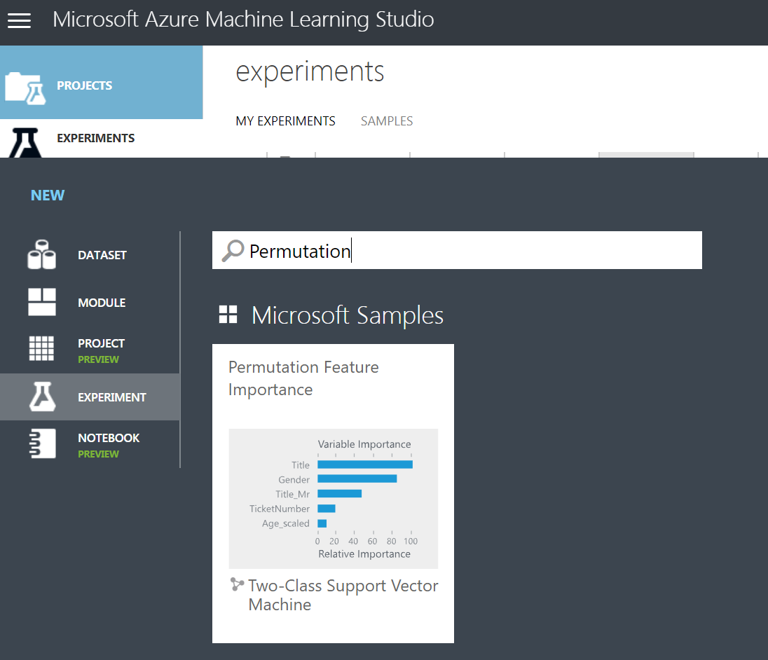
Once the workspace is opened, click on Saved Datasets and My Datasets. You will see +New button in bottom of the screen, by clicking it, you should be able to choose DATASET, then click “From Local File”. The upload of dataset dialog box will appear as below:
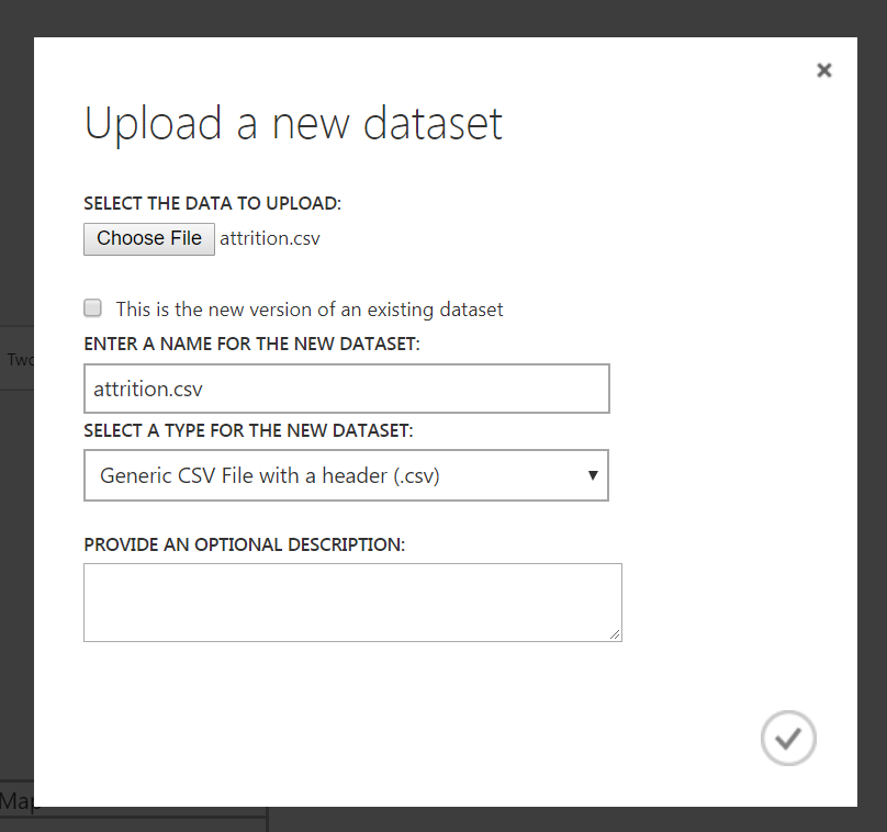
Once it’s available in the workspace, drag it to workspace.
Then, choose Feature Section and drag Filter Based Feature Selection item on the workspace. After connect the “attrition.csv” dataset to the input of FBFS, you would choose the feature scoring method to Chi Squared and choose the target column to Attrition.

Hover over FBFS box, then right click, execute Run selected. It will execute the selection. After the run, right click on the FBFS box, then select Features > Visualize and the below output is displayed.
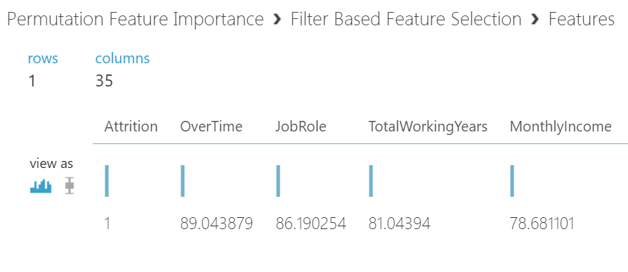
Interestingly, as with first experiment with R using correlation coefficients, it identified the overtime as the large factor.
Then from Data Transformation, choose “Select Columns in Dataset” and the workspace will now look like somewhat below,
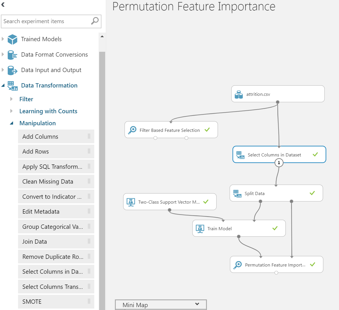
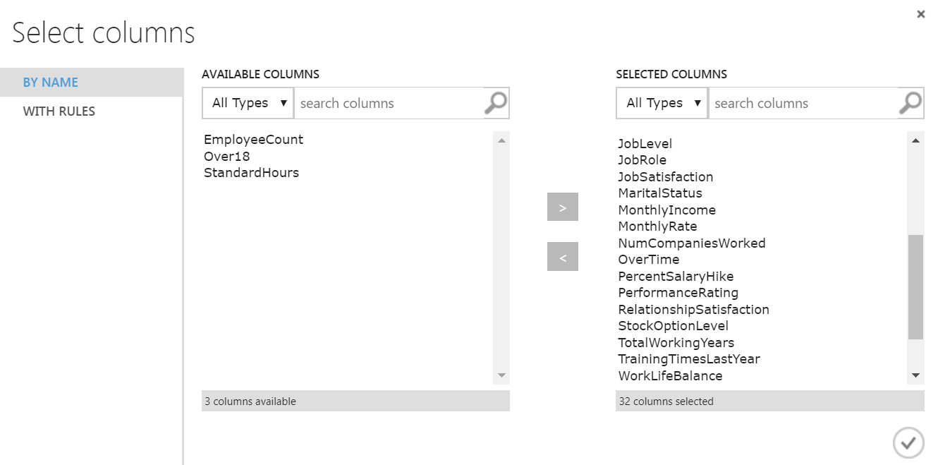
Then we will choose all the columns except EmployeeCount, Over18 and StandardHours as stated previously.
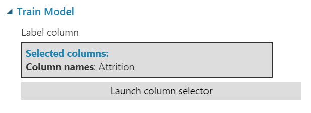
Then we will choose Train Model box, then choose the Attrition column as Label.
Finally, we will run PFI experiment. Click Run. Once it is run, the model is trained and available for review. Hover over Permutation Feature Importance then right click as below:
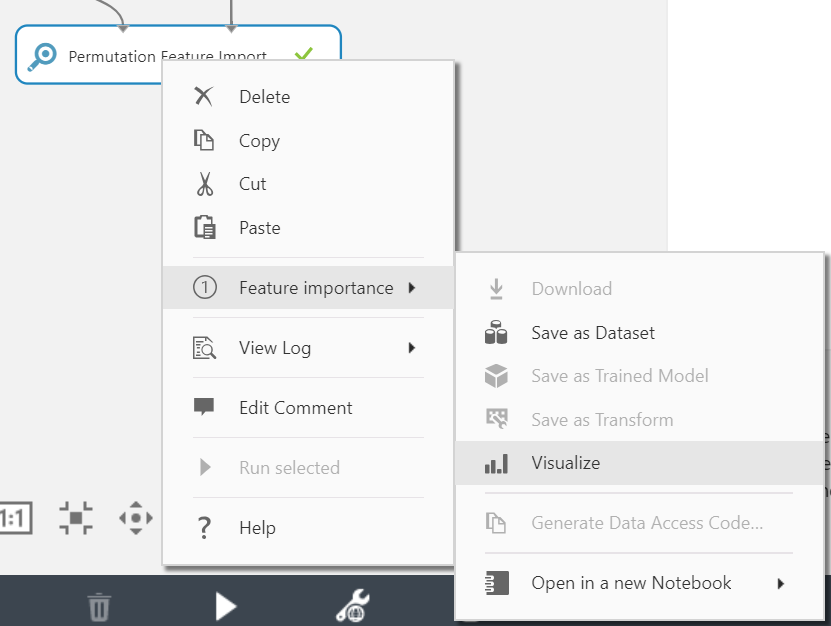
Once you click Visualize, we should be able to see the PFI report as below.
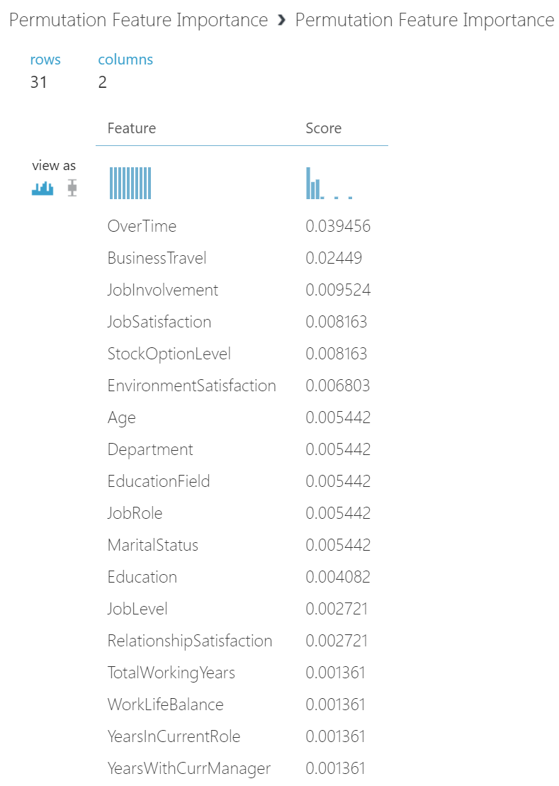
What does the above PFI findings highlight? Perhaps we can come to below observation:
| Top 4 Features | Initial Observation |
| Overtime | Higher reported Overtime, employees are more likely to leave. |
| Business Travel | More travel requirements may result more likely to leave. This observation may be tied to job roles and can be challenging for company to address. |
| Job Involvement | Employees consider their level of job involvement seriously and those may not feel involved are more likely to leave |
| Job Satisfaction | As tied to “Job Involvement” feature, employees consider their job satisfaction seriously and those unsatisfied are more likely to leave |
Again, as stated before, this should not be looked as if de-facto conclusion in regard to attrition. However, it’s interesting to note of top concern of “Overtime” agreed with R implementation of correlation coefficients. If you would like to find out more on this powerful experiment, please read about permutation feature importance.
Wrap Up
I find that machine learning experiment’s results are always interesting and somewhat unexpected in certain cases. On this comparison, the feature ranking results of PFI are often different from the feature selection statistics that are utilized before a model is created. This is useful in many cases, especially when training “black-box” models where it is difficult to explain how the model characterizes the relationship between the features and the target variable.
We encourage everyone try this out and apply various statistical modules and machine learning models. In upcoming blog, I plan to bring out how we can achieve similar implementation applying the PFI from ML.Net and comparison reports with this blog.

0 comments