MongoDB to Azure Cosmos DB for NoSQL Migration – Learnings from Java SDK V4 Micro-Optimizations

Subhasish Ghosh

Theo van Kraay

February 22nd, 20240 2

The authors wish to thank Govind Kanshi (Principal PM Manager), Abinav Rameesh (Principal PM Manager), Kushagra Thapar (Principal Engineering Manager), Annie Liang (Sr. Software Engineer) and Faiz Chachiya (Sr. Cloud Solution Architect, CSU) for their valuable insights, and contributions during the Proof-of-Concept (PoC).

Introduction

Azure Cosmos DB is Microsoft’s premier fully managed NoSQL database for modern app development. It is ideal for solutions including artificial intelligence, digital commerce, Internet of Things, booking management and other types of use cases. It offers single-digit millisecond response times, automatic and instant scalability along with guaranteed speed at any scale.

This blog post outlines the migration approach and Azure Cosmos DB for NoSQL Java SDK V4 micro-optimizations the team undertook while attempting to migrate an existing on-premises MongoDB database hosting a centralized Fraud Analytics platform to Azure Cosmos DB for NoSQL at a large Retail customer. The post highlights the PoC performance benchmark requirements, the challenges faced, and the resolution steps undertaken to achieve the PoC goals.

Use case & background

The customer is a retail corporation with a combination of both offline & online ecommerce business models. With 100 Million+ unique visitors per month, the eCommerce architecture is a classic event-driven, loosely coupled, microservices architecture.
The centralized fraud detection and analytics platform has a front-end capturing fire-and-forget transactional events which are then fed into a CQRS (Command and Query Responsibility Segregation) pattern-based dedicated databases. A MongoDB Cluster in an on-premises DC hosts multiple MongoDB databases.
The Database for our PoC is referred to as Grade. Grade is essentially a time-series aggregate MongoDB database capturing approximately 5,000+ parameters which are parameterized on specific user-defined rules.
Pre-calculated aggregates are created and stored which include SUM, MIN, MAX, across a specific customer, email, address etc. across a period of minimum of 36 hours to maximum of 9 months.
The purpose of this database is to answer pinpointed queries like, how much in USD did a customer named Subhasish spend on a specific SKU in the past 72 hours? The database is fine-tuned for a high-volume, sudden-burst scenario which are typical in eCommerce Holidays (e.g., Black Friday, Cyber Monday, Christmas & New Year sales etc.).
The primary query is to fetch various grade metrics history based on the indexed unique key. E.g., the following query returns all previous day’s records for a customer named Subhasish.

db.collection.query({key: 'Subhasish', date: '2023-07-11'})

Peak throughput estimate during primary Holiday Season sales event: Reads: 100-120K ops/sec, Writes: 200-250K ops/sec

A high-level block diagram of the architecture is exhibited below:

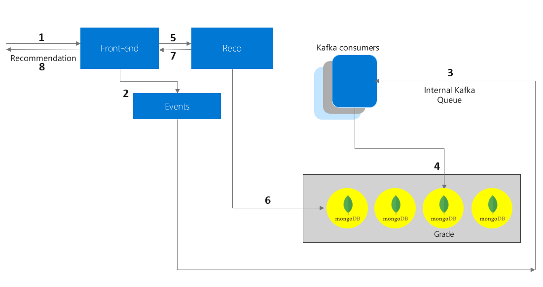
The entire flow is real-time since we cannot have aggregates getting calculated in real-time when the actual OLTP system is handling massive volume of transactions and a customer’s order is pending confirmation in real-time since the fraud analytics system recommendation is yet to come through. In summary, this solution is highly latency sensitive.

Performance benchmarks

Table below captures the expected latency in the PoC post re-modeling from MongoDB to Azure Cosmos DB for NoSQL:

Operation	Average	P95	P99	App-entry point on VM	Max Queries / sec (qps)
Point-read	< 3 ms	< 10 ms	< 50 ms	1	3,000
In-partition Query	< 7 ms	< 15 ms	< 50 ms	1	3,000
Upsert	< 3 ms	< 5 ms	< 10 ms	1	3,000

The crux of the PoC was to achieve a performance benchmark of requestLatency of 1 or 2 ms (i.e., < 3 ms) for point-reads of 0.2 KB item size from a single App-entry point hosted on an Azure virtual machine (VM) for a period of 1 hour consistently at 3,000 qps. The term requestLatency refers to how long a CRUD operation took. It represents a round trip time as observed by the client including retries (if any). The VM configuration was 8 vCores / 27 GB.

Re-modeling from MongoDB to Azure Cosmos DB for NoSQL

The original MongoDB data design involved storing data for each unit in a separate MongoDB replica set. Each grade/parameter is stored in a separate collection. Time_bucket is an integer which represents hour/days/etc. since the epoch. Primary access pattern is write-heavy for this database, with primary operation being update() with $inc op. In MongoDB, you basically insert a new document if no match exists (upsert) with option upsert: true:

If document(s) match query criteria, db.collection.update() performs an update.
If no document matches the query criteria, db.collection.update() inserts a single document. And $inc update operator basically increments a field by a specified value.

Sample item schema in MongoDB:

{ key,  time_bucket,  value }
Subh    2023-05-01    11.51
Subh    2023-03-01     9.00
Subh    2023-06-04   200.88
…
…
Aayushi 2023-02-20     5.00
Aayushi 2023-04-01    15.00

In Azure Cosmos DB for NoSQL, all Grade collections for a given time unit in MongoDB basically translate to a single container in CosmosDB. A time bucket record basically has a synthetic partition key (pk) which is created by concatenating multiple properties of an item. This ensures we get an even distribution of data for a given Grade type, as well as across all Grade types. A sample JSON schema for an item:

    pk: < Domain | GradeName | TimUnit | Key >
    id: < TimUnit >
bucket: < Date >
   val: < number >
   ttl: < secs to expire >

A sample input document using the above schema:

    pk: ssp.com|cust_ord|Day|125636751>
    id:  18813
bucket:  <Date>
   val: 192.33
   ttl: 120

In our example above, com is domain, cust_ord is GradeName, Day is the time-unit bucket, and finally, 125636751 is the key identifying a specific customer. Id represents time-bucket represented as an integer value of time units since epoch. An important point to note is that all records for a given key will land in the same logical partition. Thus, for a given grade parameter say, cust_ord, all records for this specific customer 125636751 will reside on the same logical partition.

Partition key model in Azure Cosmos DB for NoSQL

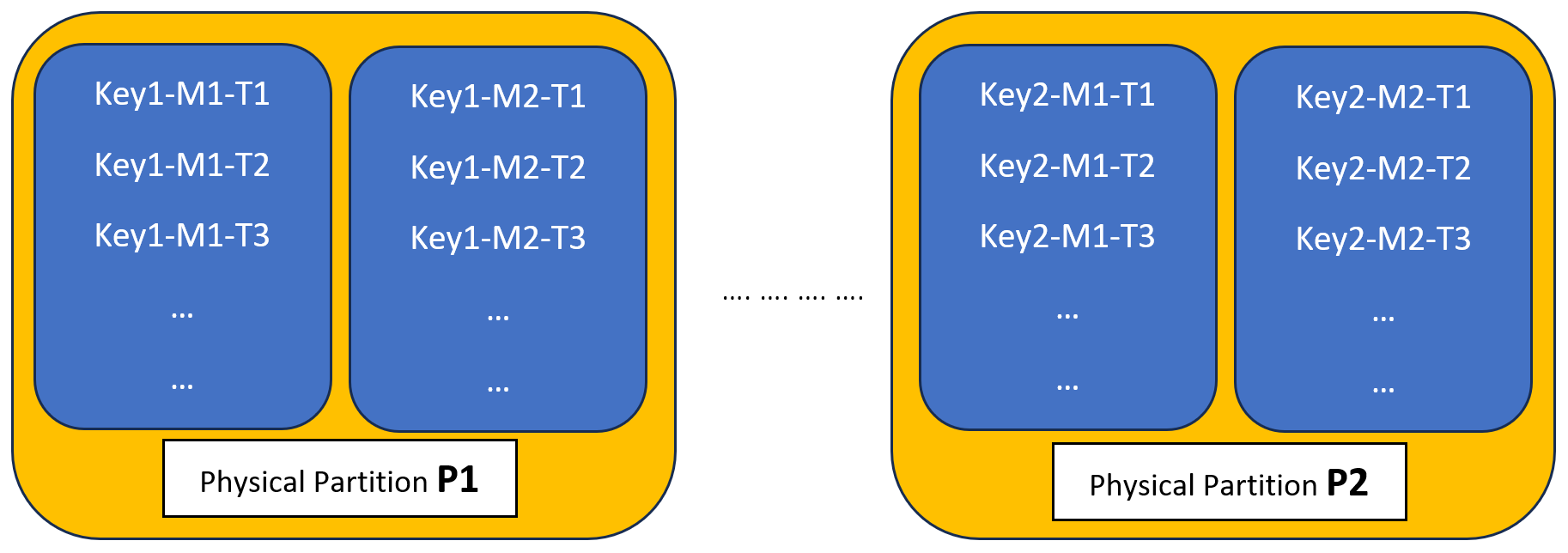
Each Key resides in a unique partition.
Each [GradeN] and associated bucket records reside within the partition.
A single query fetches all grades and associated bucket records in a partition.

Functional Tests

For our test purposes, we used the following setup:

An Azure Cosmos DB for NoSQL container with a throughput of 20,000 RU/s
Item size of 0.2 KB
Operations primarily to be tested: point read and upsert
5,000 async writes including 40% creates and 60% increments (using Patch API)
10 threads
Java SDK v4 4.36.0 // Replace with the latest version in your test
Account configured with Direct Connectivity mode, Session Consistency
Test VM: South Central US
Azure Region hosting Azure Cosmos DB: South Central US
GitHub repo with sample schema, settings and load test code in Java can be accessed here

Recommended best practice is to always use the latest Java SDK V4. For your tests, replace Java SDK version with the latest version.

Challenges

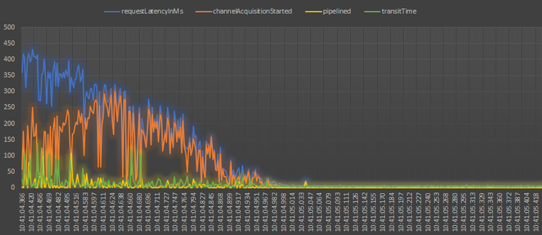
Challenge #1: P99 requestLatency on create/patch was 300+ ms at 500 qps: How to diagnose and troubleshoot?

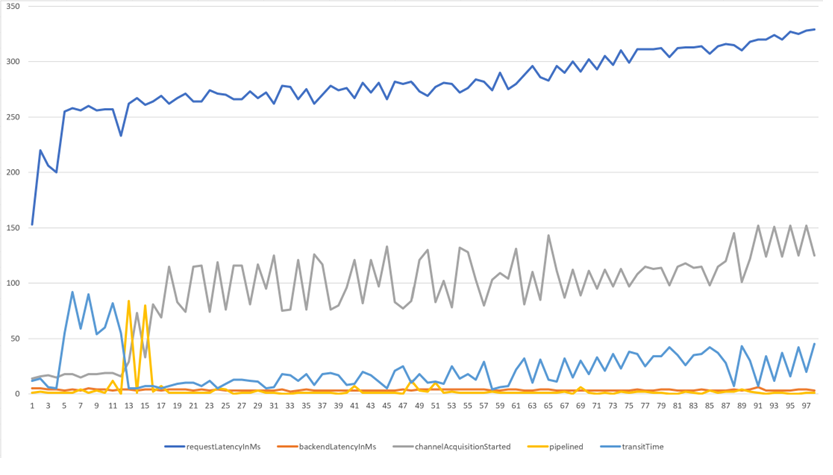
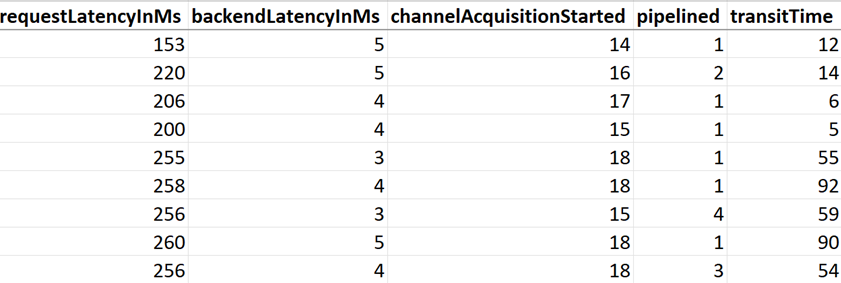
Resolution: Recommended practice is to proactively leverage Azure Cosmos DB for NoSQL Java SDK V4 client-side Diagnostics during dev/test stage of a PoC. Azure Cosmos DB for NoSQL Java SDK V4 enables you to extract and represent information related to database, container, item, and query operations using the Diagnostics property in the response object of a request. This property contains information such as CPU and memory levels on the compute host for the SDK instance as well as service-side metrics covering nearly every aspect of the execution of your request. The JSON output could be used effectively to undertake proactive custom conditional client-side monitoring & in-depth troubleshooting of commonly found client-side issues. In our PoC, diagnostics provided visibility into transport layer events, a sample plot is as exhibited below:

Additionally, review of systemCpuLoad property in systemInformation section of the diagnostics JSON output showed consistently high CPU (75%+) during creates. Firing 100’s of create calls (async API) in a loop non-stop generated high CPU load.

"systemCpuLoad":"
    (2022-05-02T07:27:59.495855600Z 79.0%),
    (2022-05-02T07:28:04.489517300Z 75.0%),
    (2022-05-02T07:28:09.495177300Z 78.0%),
    (2022-05-02T07:28:14.495187100Z 79.0%).

We concluded that executing 100’s of create calls (async API) in a loop non-stop is generating too much pressure on the Java SDK V4 underlying Reactor library. We added a 1-ms delay between each async create call in the loop. This improved the CPU load on the client-machine, and we observed single-digit ms on create and patch calls.

Below stats are from 5000 calls to API createOrIncrement – which first attempts to create an item and if it fails, does a patch / increment operation:

createOrIncrement (ms)      [count: 5000, avg:   9 | min:  4, max:  421 | med:   8, 95%:  10]

---------------------------------------------------------------------------------------------

  |-create (ms)             [count: 1814, avg:   7 | min:  4, max:  385 | med:   6, 95%:   8]

---------------------------------------------------------------------------------------------
  |-create conflict (ms)    [count: 3186, avg:   2 | min:  1, max:  328 | med:   2, 95%:   3]

  |-patch (ms)              [count: 3186, avg:   6 | min:  5, max:   65 | med:   6, 95%:   7]

Learning #1: Pro-actively leverage Azure Cosmos DB for NoSQL Java SDK V4 Diagnostics conditional logging for diagnosing latency related issues early-on into development.

Challenge #2: At 900 qps, we received high channelAcquisitionStarted times in creates. This negatively impacted our ability to push queries further.

Resolution: In an attempt to scale from 500 qps to 1,000 qps and determine max throughput that is achievable by 1 VM, we received high channelAcquisitionStarted times at around 900 qps as exhibited below.

The transportRequestTimeline section of the Diagnostics JSON output provides essential information on the specific transport layer events since the CRUD request was fired. The channelAcquisitionStarted event denotes we have successfully queued the request, and now all we need is for us to acquire a channel which will enable to send the request to the actual endpoint. The endpoint here refers to the full rntbd (Microsoft TCP layered stack) FQDN address including partition & replica IDs. A channel is a connection from your client VM to Azure Cosmos DB machine which hosts the replica to which this request is now going to be transported.

We customized connCfg rntbd network connectivity parameters for Azure Cosmos DB via Azure Cosmos DB Java SDK V4.

"connCfg":{
         "rntbd":"(cto:PT5S, nrto:PT5S, icto:PT0S, ieto:PT1H, mcpe:130, mrpc:30, cer:true)",
         ………………………………
         ………………………………
         },

Read this blog post for a detailed analysis of the individual parameters and suggested connCfg values based on different read and write optimized eCommerce use-cases.

In the above, cto stands for ConnectionTimeout duration on the rntbd TCP stack for a given CRUD request (in our use-case scenario, it is for the create operation). This signifies that in case you are facing any connectivity issues, you are instructing the TCP stack to retry that specific request after a customized time duration interval. By default, cto is set to 5 seconds by the Java SDK V4. For specific use-cases you can choose to customize it. E.g., if you are running an eCommerce site which is expecting to observe a high volume of peak requests during a Black Friday event, you can choose to customize the cto values based on the query patterns in your code. Here are some example values we’ve observed customers using:

1. Read heavy app primarily doing point-reads: 600 ms
2. Read heavy app primarily doing in-partition queries: 600 ms
3. An app primarily executing stored procedures: 1 sec
4. Write heavy app: 600 ms
5. An app which does cross-partition queries: 5 sec
6. An app which primarily does Cross Region calls: 1 Sec

Initial setup was changed from cto = 5 seconds

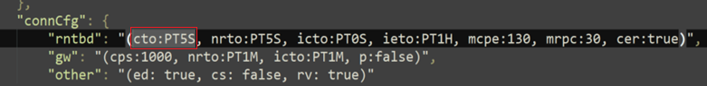
To cto = 600 ms (0.6 seconds)

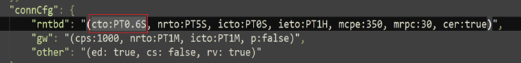
/* Exercise caution in production environments.
/* Reach out to Microsoft for specific guidance.
DirectConnectionConfig directConnectionConfig = DirectConnectionConfig.getDefaultConfig();
directConnectionConfig.setConnectTimeout(Duration.ofMillis(600));
directConnectionConfig.setNetworkRequestTimeout(Duration.ofSeconds(5));
directConnectionConfig.setIdleConnectionTimeout(Duration.ofSeconds(0));
directConnectionConfig.setIdleEndpointTimeout(Duration.ofHours(1));
directConnectionConfig.setMaxConnectionsPerEndpoint(350);
client = new CosmosClientBuilder()
         .endpoint(AccountSettings.HOST)
         .key(AccountSettings.MASTER_KEY)
         .consistencyLevel(ConsistencyLevel.SESSION)
         .contentResponseOnWriteEnabled(false)
         .directMode(directConnectionConfig)
         .buildAsyncClient();

Additional Tip:

In addition to the above, you can leverage an end-to-end timeout policy feature in Java SDK V4. An end-to-end timeout policy is specifically catered to solve challenges related to tail latency which effectively cause availability to drop significantly since requests are not being cancelled. You provide a timeout value that covers the whole execution of any request, including requests that span multiple partitions. Ongoing requests will be cancelled if the timeout setting is reached. The timeout duration can be set on CosmosItemRequestOptions. The options can then be passed to any request sent to Azure Cosmos DB. Read this blog post for more information and sample code for enabling this feature.

The above two changes lowered our channelAcquisitionStarted times for bulk of our queries, thereby positively impacting the round-trip latency.

Learning #2: Review your use-case and customize the connCfg rntbd network connectivity parameters in Azure Cosmos DB using Java SDK V4.

Challenge #3: At 1,500 qps, we received high channelAcquisitionStarted times in creates. This negatively impacted our ability to push queries further.

Resolution: In an attempt to further optimize and lower channelAcquisitionStarted times at around 1,300-1,500 qps, we upgraded SDK from 4.36.0 -> 4.42.0 (the latest stable version of the Java SDK available during the time of the PoC) which allowed us to use openConnectionsAndInitCaches API. This API allows us to set CosmosContainerProactiveInitConfig value for implementing proactive connection management. This feature, added to the Java SDK in Feb 2023, enables warming up connections and caches for containers for both the current and read region and a pre-defined number of preferred remote regions, as opposed to just the current region. This feature is especially useful in a few scenarios wherein improving the tail latency in cross-region failover scenarios and reducing overall latency for writes in a multi-region scenario wherein only a single write region is configured. Read this blog post for more information and sample code for enabling this feature.

A point noteworthy is that the proactive connection regions are a subset of the preferred regions configured through the CosmosClientBuilder. The first getProactiveConnectionRegionsCount() read regions from preferred regions are picked.

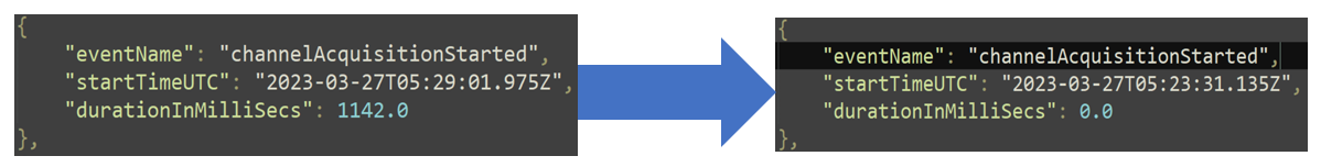
This change assisted in lowering the request latency from earlier observed numbers and solved channelAcquisitionStarted durationInMilliSecs for a large batch of queries.

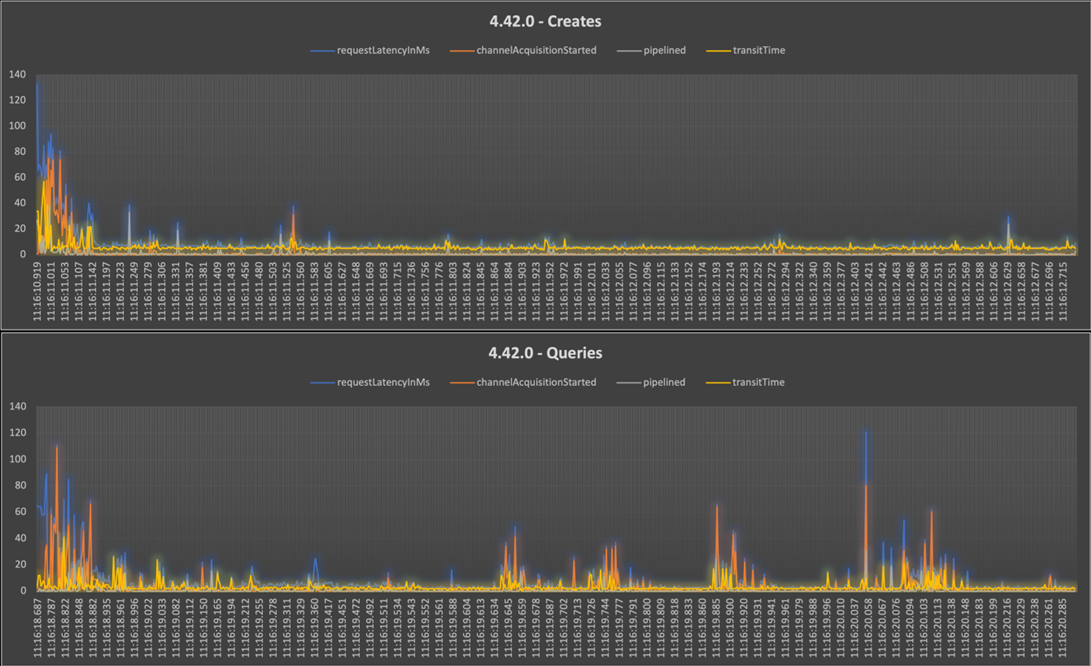
E.g., one of the worst performing queries at 1,142.0 ms reduced to 0.0 ms post incorporation of this change.

Additional Tip:

A new threshold-based parallel processing capability in the Java SDK has also been added, which can be activated when creating an end-to-end timeout policy explained in one of the earlier sections, to improve tail latency and availability even further. When enabled, parallel executions of the same request (read requests only) will be sent to secondary regions, where the request that responds fastest is the one that is accepted.

Assume you have three regions set as preferredRegions in CosmosClientBuilder, in the following order: East US, East US 2, South Central US.

Assume the following values for speculation threshold and threshold step:

int threshold = 500
int thresholdStep = 100;

At time T1, a request to East US is made.
If there is no response in 500ms, a request to East US 2 is made.
If there is no response at 500+100ms, a request to South Central US is made.

Read this blog post for more information and sample code for enabling this feature.

Learning #3: Leverage Azure Cosmos DB for NoSQL Java SDK V4 specific properties for query optimization and improving tail latencies.

Challenge #4: How to scale from 1,500 qps to 3,000 qps for achieving 2 ms requestLatency using Java SDK V4?

Resolution: The above-mentioned three learnings enabled us to lower P99 requestLatency from 300 ms+ to avg. 50 ms consistently for both point-reads and in-partition queries. To optimize further to reach 1 or 2 ms average latency for point-reads, we undertook two micro-optimization steps:

Step1: We undertook an application code analysis. Azure Cosmos DB for NoSQL Java SDK V4 is based on Project Reactor and Project Netty library. Designed for reactive programming, the Async API sends requests to Azure Cosmos DB for NoSQL using Reactor Netty with async I/O at the OS level – no block waiting for the responses. This allows us to push out as many requests per second as your system hardware and your provisioned throughput allows. The reactive streams allow asynchronous stream processing by scheduling tasks on worker threads. We did a comparative performance code analysis on the same Flux and observed performance difference between the two available Project Reactor Schedulers: subscribeOn and publishOn.

We switched from default .subscribeOn to .publishOn owing to publishOn offsetting the blocking work on a separate thread. A sample transformation is exhibited below:

public static void createRecordAsync(final CosmosAsyncContainer container, final String pkey, final String id) {
    try {
        // …… //
        container
                .createItem(day, new PartitionKey(pkey), options)
                // .subscribeOn(Schedulers.boundedElastic())
                .publishOn(Schedulers.boundedElastic())
                .doOnSuccess(response -> {
                    // …… //
                    double requestCharge = response.getRequestCharge();
                    Duration requestLatency = response.getDuration();
                    System.out.println(response.getDiagnostics().toString());
                    //System.out.println("\n\n\n");
                })
                .doOnError(error -> {
                    error.printStackTrace();
                })
                .subscribe();
    } catch (CosmosException ce) {
        ce.printStackTrace();
    }
}

Since our use-case is predominantly targeted towards optimizing non-blocking calls, using subscribeOn means running the initial source emission e.g., subscribe(), onSubscribe() and request() on a specified scheduler worker. This is also the same for any subsequent operations, e.g., onNext/onError/onComplete, map etc. and no matter the position of subscribeOn(), this behavior would happen. In summary, subscribeOn forces the source emission to use specific Schedulers.

On the other hand, using publishOn changes Schedulers for all the downstream operations in the pipeline. This change of task execution context for the operations in the downstream using .publishOn(Schedulers.boundedElastic()) uses a thread pool containing 10 * number of CPU cores of your app entry point (in our use-case, Azure VM). This is an excellent choice for optimizing IO operations or any blocking call.

Flux<Integer> flux = Flux.range(0, 2)
       .publishOn(Schedulers.boundedElastic());

This solved our on-going latencies and dropped P99 < 10 ms.

Step2: Our application code was using the Scatter Gather pattern in Java that allows you to route messages to a number of dynamically specified recipients and re-aggregate the responses back into a single message. We replaced Scatter method with subscribe() when issuing each query within the loop. Instead of collecting all 1,500 query fluxes and firing at once using Scatter Gather pattern, we made the following change:

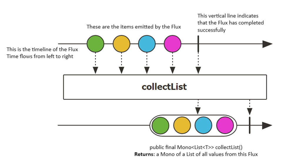
// Initially, we were firing all fluxes at about the same time and collecting results (Java Scatter-Gather pattern)
Flux.merge(fluxes).collectList().subscribe(//your method here);

// We changed to:
Flux.merge(mono).collectList().subscribe(//your method here);

Here, the merge function executes a merging of the data from Publisher sequences contained in an array into an interleaved merged sequence. We do a collectList() which accumulates the sequence emitted by this Flux into a List that is emitted by the resulting Mono when this sequence completes.

The above-mentioned micro-optimizations resolved our on-going latencies and dropped avg. latency for point-reads < 3 ms. Additionally, the performance held consistently over a duration of a few hours, when we scaled from our initial 1,500 qps to 3,000 qps. Finally, we subjected the Test setup for spike testing by scaling the same set of queries (point-read, query and upsert) for max qps to 50,000 (across multiple entry-points) in a sporadic fashion to mimic real-life eCommerce sales event scenarios (e.g., Black Friday sales event). The above micro-optimizations allowed us to achieve similar results thereby satisfying the desired outcome in the tests.

Learning #4: Leverage appropriate Reactive non-blocking patterns in code to reduce tail latency and further optimize execution latency down to a single-digit millisecond.

Summary of Learnings

Learning #1: Pro-actively leverage Azure Cosmos DB for NoSQL Java SDK V4 Diagnostics conditional logging for diagnosing latency related issues early-on into development.
Learning #2: Review your use-case and customize the connCfg rntbd network connectivity parameters in Azure Cosmos DB using Java SDK V4.
Learning #3: Leverage Azure Cosmos DB for NoSQL Java SDK V4 specific properties for query optimization and improving tail latencies.
Learning #4: Leverage appropriate Reactive non-blocking patterns in code to reduce tail latency and further optimize execution latency down to a single-digit millisecond.

Conclusion

Azure Cosmos DB for NoSQL offers single-digit millisecond response times, automatic and instant scalability along with guaranteed speed at any scale. Best practices for using Azure Cosmos DB for NoSQL Java SDK V4 allow you to improve your latency, availability and boost overall performance. Leveraging the latest Java SDK V4 coupled with specific SDK level optimizations is advisable if you have high performance and low latency scenarios as covered in our blog post. Do reach out to the Azure Cosmos DB Product team for specific insights into your use-case scenario.

Let us know your thoughts in the comments section below.