
R is a programming language that is widely used by data scientists, and developers seeking a more powerful tool to work with data. While data scientists use R to write programs, their work product is rarely the program itself. Instead, they produce reports or presentations from the results generated by their R program to help influence or drive business decisions.
R Tools for Visual Studio (RTVS), currently available as a Public Preview release, is a new tool from Microsoft for creating R programs using Visual Studio. RTVS is free, and Open Sourced under the MIT license. It can be downloaded by following the instructions here, and you can read our documentation here.
If you prefer videos, here is a walkthrough of some of the top features of RTVS:
A Quick Tour of R
R is a strong, dynamically typed, interpreted language that draws a lot of inspiration from other languages. It is a functional language that heavily draws from Scheme and S. It is beyond the scope of this blog post to discuss the semantics of the language, but I strongly encourage you to read these two freely available online books for a deep introduction to the language:
The remainder of this blog post is a quick tour of R, its libraries, and RTVS with the goal of inspiring you to learn more about the language, its libraries, and how it can be a useful addition to your toolbox for analyzing data.
The quickest way to get started with R is through its Read-Eval-Print Loop (REPL), which lets you send commands interactively to the R interpreter. In RTVS, we surface the R REPL through the R Interactive Window.
As you can see, you can type 3 + 4 and have the result immediately computed by R; no compilation step necessary:
3 + 4[1] 7R’s strength is working with data. Therefore, it’s not surprising that the most heavily used data structure in R is the R dataframe, which is a convenient way of working with tabular datasets. There are many ways of getting data into an R dataframe, but perhaps the easiest is to read it from a URI. Below, you’re reading a CSV file containing data about locations of airports in the United States from Github:
usa_airports <- read.csv("https://raw.githubusercontent.com/jflam/VSBlogPost/master/usa_airports.dat", stringsAsFactors = TRUE)In R, you assign variables using the <- operator, and you invoke functions using parenthesis. So in the code above, you’re invoking theread.csv() R library function, passing in the URI to the CSV file.
You can get help on any R library function by using the ? operator from the REPL. For example, to get help on the read.csv API, just type?read.csv in the REPL.
Next, you’re using another R function, head() to display a summary of the first 5 lines of the file:
head(usa_airports) X ID name city country
1 318 6891 Putnam County Airport Greencastle United States
2 1104 6890 Dowagiac Municipal Airport Dowagiac United States
3 1121 6889 Cambridge Municipal Airport Cambridge United States
4 1470 6885 Door County Cherryland Airport Sturgeon Bay United States
5 1507 6884 Shoestring Aviation Airfield Stewartstown United States
6 1617 6883 Eastern Oregon Regional Airport Pendleton United States
IATA_FAA ICAO lat lon altitude timezone DST
1 4I7 \N 39.63356 -86.81381 842 -5 U
2 C91 \N 41.99293 -86.12801 748 -5 U
3 CDI \N 39.97503 -81.57758 799 -5 U
4 SUE \N 44.84367 -87.42156 725 -6 U
5 0P2 \N 39.79482 -76.64719 1000 -5 U
6 PDT KPDT 45.69500 -118.84139 1497 -8 A
Region
1 America/New_York
2 America/New_York
3 America/New_York
4 America/Chicago
5 America/New_York
6 America/Los_AngelesThe head function is fairly primitive, as it just generates text-based output. That’s not surprising since R has been around since 1993. Surely we can do better in 2016?
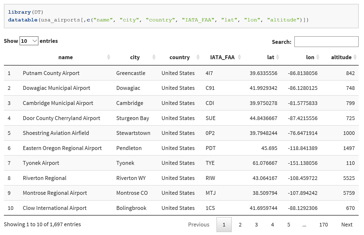
As it turns out, we can. There are a lot of libraries in R that bind the R programming language to the most powerful hardware-accelerated rendering platform on the planet: HTML. In R, this is accomplished through a set of Open Source libraries known as htmlwidgets for R. Below is the same dataframe rendered using the DataTable widget. We generate an HTML page that contains all of the data from the usa_airports dataframe, and open up a browser window using the default browser that shows an interactive table containing the data. The data really is interactive; try typing “Seattle” into the search box to see it filter the data to only airports in Seattle in real time, or click on column headings to sort by that column.
library(DT)
datatable(usa_airports[,c("name", "city", "country", "IATA_FAA", "lat", "lon", "altitude")])
(to get to the interactive table, please click on the image below)
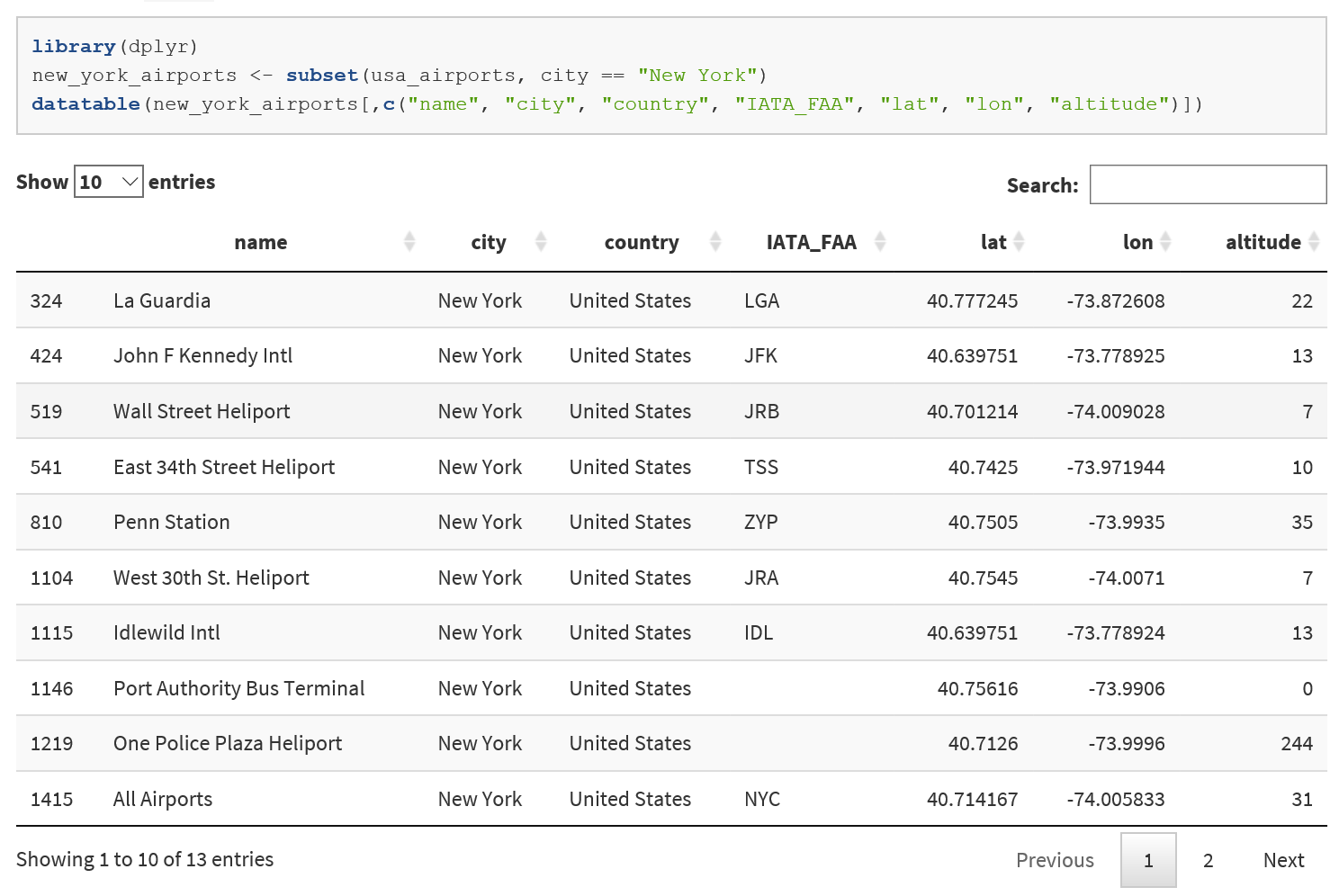
If you prefer to manipulate your data programmatically, you can easily do so as well. A popular library for manipulating data is the dplyr library by Hadley Wickham. Let’s say that we wanted to generate a list of airports located near New York city. You can do this easily via the subset function from dplyr:
library(dplyr)
new_york_airports <- subset(usa_airports, city == "New York")
datatable(new_york_airports[,c("name", "city", "country", "IATA_FAA", "lat", "lon", "altitude")])
(to get to the interactive table, please click on the image below)
You can also do more sophisticated filtering: e.g., select all the airports in NYC at below 25 feet elevation, ordering the rows by altitude and selecting only the name, altitude, latitude and longitude of the airport:
low_nyc <-
    usa_airports %>%
    filter(city == "New York" & altitude < 25) %>%
    arrange(altitude) %>%
    select(name, altitude, lat, lon)
datatable(low_nyc)
(to get to the interactive table, please click on the image below)
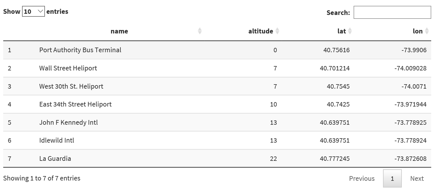
Here, you see a more sophisticated use of R syntax via the %>% or “pipe” operator. This operator lets you naturally compose operations and read them from left to right. So in the above example, you take the usa_airports dataframe, filtering all of the rows where the conditioncity == "New York" & altitude < 25 holds true, sorting the rows by the altitude column, and selecting only the columns name,altitude, lat, and lon for the result dataset which is stored in the low_nyc variable.
If you’re curious about the implementation of the pipe operator, see the magrittr package, as well as this excellent blog post on how magrittr was influenced by the forward pipe operator from F#.
Plotting data on maps
Once you have your dataset, you can plot it on an interactive map. The leaflet HtmlWidget is an excellent library for generating interactive maps. In the code fragment below, you take the dataframe that contains low altitude New York City airports that you generated via dplyr in the previous step, and using the now-familiar pipe operator send it to the leaflet library, asking it to generate map tiles and plotting circles on them using the lon and lat columns for the positions of the circles, and using the name column for the popup that appears when the user clicks on a circle.
library(leaflet)
map <-
    new_york_airports %>%
    leaflet() %>%
    addTiles() %>%
    addCircles(~lon, ~lat, popup = ~name, radius = 200, color="blue", opacity = 0.8)
map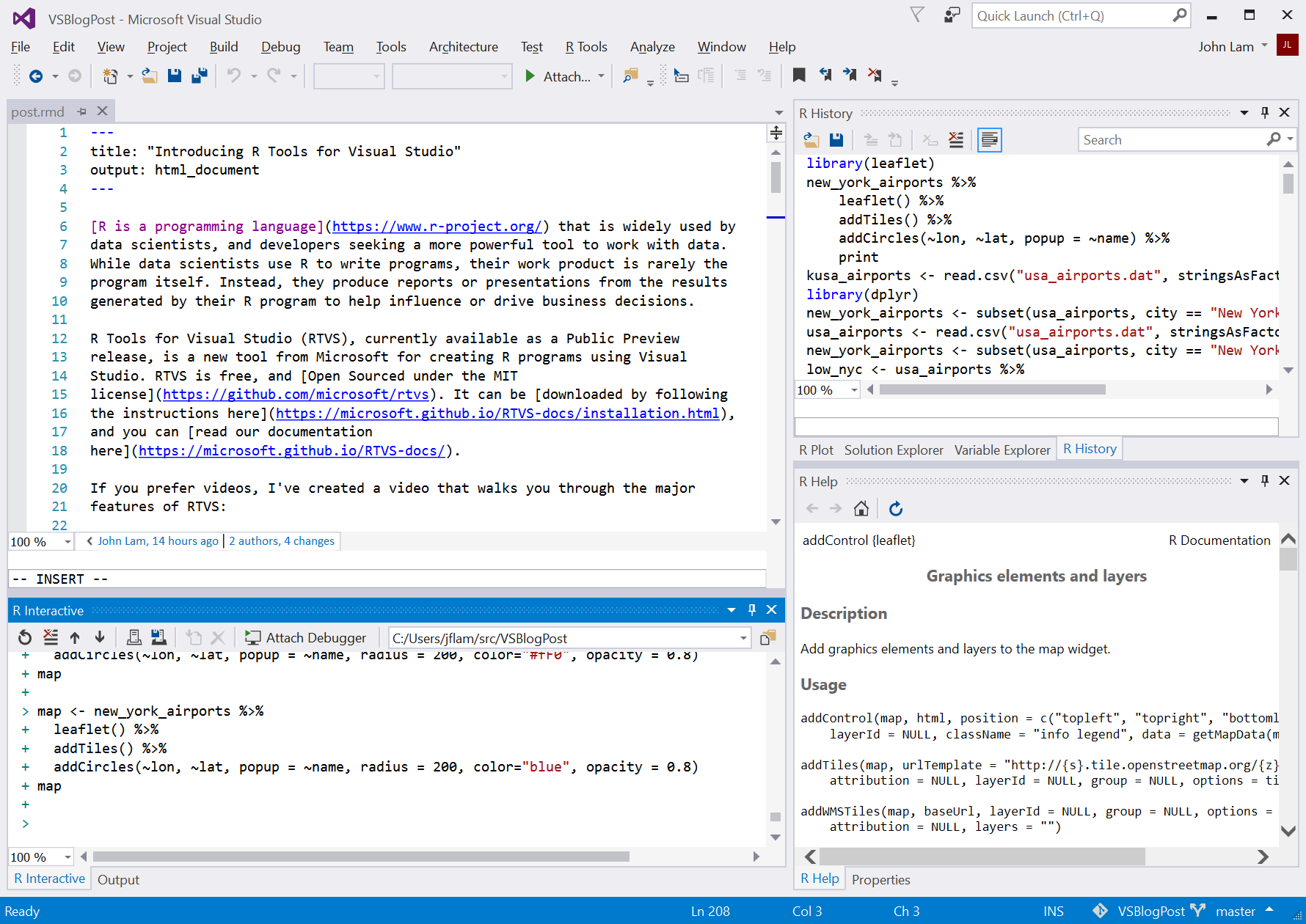
Wrapping up the tour
There is lots more to learn about R than I have time or space for in this blog post. However, hopefully what I’ve done is whet your appetite to learn more about R. There are many, many things that I haven’t covered in this blog post, so I’ve included a bunch of resources below to help you better understand R and its libraries.
Introduction to the R Programming Language
- An Introduction to R: written by David Smith, who currently works at Microsoft on the R team.
- Introduction to R Programming: a free online class created by Microsoft to help you learn R.
Key R Libraries
- dplyr is the data manipulation “d plyer” library that is a key tool for helping you quickly manipulate your data into a form that you can analyze.
- ggplot2 is a plotting library that builds on the grammar of graphics ideas by Hadley Wickham
- ggvis is a plotting library that generates plots on an HTML canvas, using the same grammar of graphics semantics as ggplot2
- rodbc lets you read data from an ODBC compliant database like SQL Server
Microsoft R products
Microsoft has a deep commitment to R, and provides a full-stack R solution for your applications, complete with tooling, runtimes and libraries.
- R Tools for Visual Studio is Microsoft’s free, Open Source tooling for R development in Visual Studio.
- Microsoft R Open is Microsoft’s cross-platform (Windows, OS X, Linux) distribution of R. It combines integration with Intel’s Math Kernel Library for accelerated linear algebra computations, as well as integration with the checkpoint package to ensure that users of your R programs will be guaranteed to be able to run your R program using the same version of the R libraries that you used to create it.
- Microsoft R Server is Microsoft’s libraries for accelerated R computation on datasets that don’t fit in system memory. It builds on top of the benefits of Microsoft R Open, and adds
One more thing …
We’ve talked about a bunch of things in this brief blog post. However, perhaps the coolest thing about this blog post is … I wrote it in Visual Studio. The document was written in RMarkdown, a dialect of the popular Markdown markup language, which supports embedding executable R code snippets within it.
If you want to look at the source code for it, you can get it at my Github.
0 comments