
Introduction
In this code story, we will discuss applications of Hierarchical Attention Neural Networks for sequence classification. In particular, we will use our work the domain of malware detection and classification as a sample application. Malware, or malicious software, refers to harmful computer programs such as viruses, ransomware, spyware, adware, and others that are usually unintentionally installed and executed. When detecting malware in a running process, a typical sequence to analyze could be a set of disk access actions that the program has taken. To analyze software without running it, we can treat series of assembly instructions in the disassembled binary as sequences to be classified in order to identify sections of the code with malicious intent. In our novel approach, we apply techniques typically used to discover structure in a narrative text to the data that describes the behavior of executables.
Hierarchical Attention Networks (HANs) have been used successfully in the domain of document classification (Yang et al. 2016, PDF). This approach is potentially applicable to other use cases that involve sequential data, such as application logs analysis (detecting particular behavior patterns), network logs analysis (detecting attacks), classification of streams, events, etc. We will demonstrate the application of HANs for malware detection both statically (executable binary analysis) and dynamically (process behavior analysis). The supporting code uses Keras with Microsoft Cognitive Toolkit (CNTK) as the backend to train the model.
This work was inspired by our collaboration with Acronis and the services that they provide to ensure backup data stays safe.
Data
We will use two publicly available datasets to illustrate our approach and results.
The first, CSDMC 2010 API, is a sequence corpus that was also used in a data mining competition associated with ICONIP 2010. This dataset contains Windows APIs calls from malware and benign software.
For simplicity, the CSDMC 2010 dataset contains only the names of Windows APIs called by a running process. The set contains class labels for each sequence corresponding to a complete running process instance. However, we will consider the classification performance for both sequences of API calls as well as the overall trace/process.
Microsoft Malware Classification Challenge at WWW 2015/BIG 2015 dataset. It contains a collection of metadata manifests from 9 classes of malware. The metadata manifests were generated using the IDA disassembler tool. These are log files containing information extracted from the binary, such as a sequence of assembly instructions for function calls, strings declarations, memory addresses, register names, etc.
For demonstration purposes (and keeping training time to minutes on NVIDIA GeForce GTX 1060) we used hundreds of malware examples for class 1 and class 2 only. The full dataset size is 0.5 TB. However, the sample code provided in this Jupyter notebook supports multiple classes. The disassembled binary executable dumps in the Microsoft Malware Classification dataset are composed of sequences of operations and operands of unequal length, one operation per line. We will analyze the content as sequences of tuples of fixed length, considering only a number of fields extracted from each line in each experiment. For example, tuples of one field will include the operation code only, tuples of two fields will contain the operation code and the first operand, etc. Classification performance will be considered per sequence as well as for the overall executable.
What is a Hierarchical Attention Neural Network?
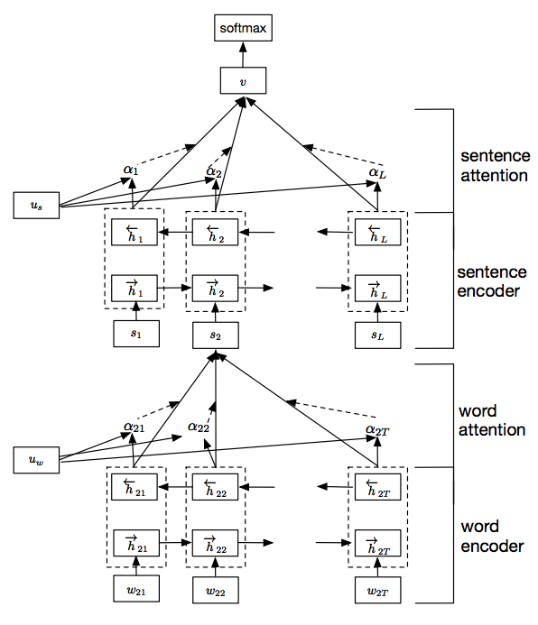
Yang, Zichao et al. proposed a HAN for document classification, presented at NAACL 2016. The solution leverages the hierarchical structure of a document, from words to sentences to documents, mirrored in a multi-layer recurrent neural network with special attention layers applied at the word and the sentence levels. The architecture of the HAN is shown in the figure below. The overall process is nicely described in detail in this blog post.
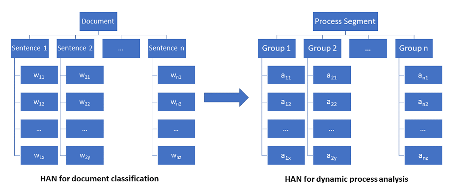
Our goal is to apply the natural language processing (NLP) inspired approach to a different domain by leveraging the sequential nature of their data: for example, classifying dynamic process behavior (sequence of API calls) or classifying malware binaries (sequence of assembly instructions).
Considering the dynamic process analysis scenario where the goal is to detect malware in a running process, a HAN-based solution will leverage the multi-layers of memory to understand the sequence of observed process actions. Classifying patterns of process behavior could then be viewed as classifying documents. Here, the sequence of process actions are analogous to a sequence of words in a text, and groups of actions are analogous to sentences.
Code walkthrough
The HAN code we provide in this Jupyter notebook is based on the LSTM HAN implementation found in this GitHub repo by Andreas Argyriou, which in turn was based on Richard Liao’s implementation of hierarchical attention networks and a related Google group discussion. The notebook also includes code from the Keras documentation and blog as well as this word2vec tutorial.
Our code extends the base notebook to support random and per-process stratified sampling, down/up-sampling of classes (binary classes only), learning hyper-parameter tuning, per-sequence and per-process evaluation metrics, configurable tuples and vocabulary sizes, extended data ingestion, configurable training environment, and other modifications to support our experimentation needs.
Important notes
- Data format: The code requires that “words” in your sequences are separated by whitespaces (tabs, spaces).
- Pre-processing: If your original data source (log/trace file, disassembled code) has a huge vocabulary, consider normalization during pre-processing and/or limiting the tuple length and vocabulary size by frequency while training. Huge “usually” means more than 5-20K. Watch out for things that can “explode” your vocabulary: GUIDs, hex addresses, temp file names, IP addresses.
- The number of words per sentence and number of sentences in a document are configurable in the code.
- It’s assumed that input uses token “<eos>” as an end-of-input sequence separator. Each input will be further broken down into sequences (documents) composed of multiple sentences as the unit of classification in the HAN training code. It is important to indicate the last sequence for a given input to avoid mixing content from different inputs. Groups (sub-sequences) of actions are treated as sentences.
- Word embeddings can be initialized using pre-trained vectors or left uninitialized. This behavior is defined by the parameter USE_WORD2VEC.
- Other configurable options define various parameters such as network dimensions, learning hyper-parameters, data sampling options, and other training environment settings.
- Deep learning framework: We use Keras with a CNTK backend, with GPU support.
The following is a high-level walk-through of the main parts of the code. For more details refer to the documentation included in the Jupyter notebook available here.
- Configure the training environment by setting the global parameters. These include: – MAX_SENT_LEN : the number of words in each sentence (a word in any token appearing in a process action tuple). – MAX_SENTS : the number of sentences in each document. – MAX_NB_WORDS : the size of the word encoding (number of most frequent words to keep in the vocabulary). – MIN_FREQ: minimum token frequency to be included in vocabulary. The final vocabulary size is the effective minimum size after considering the token dictionary, MAX_NB_WORDS and MIN_FREQ settings. – Training and test sampling strategy: randomized or stratified by process. – USE_WORD2VEC: initialize the network using pre-trained word2vec embedding weights. Note that during our experimentation, word2vec weights did not have much impact on the model performance when training for 5+ epochs. They only accelerate the learning rate in the initial epochs. – Set the network layer sizes (EMBEDDING_DIM, GRU_UNITS and CONTEXT_DIM). – Set learning hyper-parameters (REG_PARAM, LEARN_RATE, BATCH_SIZE and NUM_EPOCHS).
-
Ingest the data files corresponding to each class. The ingestion function get_sequences() breaks the input lines into tokens, sentences, and sequences according to the configured parameters. It also sets the required label per ingested sequence in the input file.
- Transform the data into the 3D format required by the network.
- Initialize the word embedding weights (if this optional step is selected).
- Build the network according to the configured layer sizes and the vocabulary size. Note that a large vocabulary will increase the size of the trained model considerably. For example, model size may vary from 2-3 MB to 80+ MB with a vocabulary size of a few hundred to several thousands of unique tokens.
- Sample and split the data into training and test datasets.
- Train the HAN network and report training and validation metrics.
- Evaluate model performance on the test set and report the classification performance per-sequence, i.e., chunks/subsets of the process actions.
- Report the overall per-process performance using a simple majority label vote (i.e., assign the most frequent per-sequence label to the process and evaluate the metrics accordingly). Other per-process heuristics may be applied according to the application needs. For example, in a dynamic process analysis scenario, one may choose to abort the process as soon as a certain threshold number of malign sequences are detected.
Dynamic malware detection: API calls classification
We are now ready to use the CSDMC 2010 API sequence corpus to classify malware vs benign software based on their API call history. For preprocessing you’ll need to save data for malware and benign sequences in separate files: malware.txt and benign.txt. The label column needs to be removed. Next separate traces with an “<eos>” token – every row in the source file corresponds to one full trace and will be broken down into segments of configurable length, corresponding to documents or sequences.
Since the CSDMC 2010 dataset contains only the API names with no additional arguments, we only have one field per action line. We split the dataset into training and validation sets using a 90/10 stratified sampling so that all sequences belonging to a trace go to either the training or the validation set for an unbiased evaluation. This resulted in a training set containing 23,470 sequences and 3,195 validation sequences.
A sample Jupyter notebook is available here. The solution in the notebook is more generalized and supports any number of fields per API call. It is a simple adaptation of the base solution provided here. Pre-processed training datasets are provided in the “data” subfolder.
The following is a sample training and validation run using sentences of 20 tokens (API calls) each, aggregated in groups of five sentences per sequence:
 =========================================================================
 Training using CSDMC dataset - No word2vec
 MAX_FIELDS = 1 - MAX_SENTS = 5
 MAX_SENT_LENGTH = 20 * MAX_FIELDS = 20
 Vocab size = 316 unique tokens
 _________________________________________________________________
 Layer (type)                 Output Shape              Param #
 =================================================================
 input_4 (InputLayer)         (None, 5, 20)             0
 _________________________________________________________________
 time_distributed_2 (TimeDist (None, 5, 200)            126700
 _________________________________________________________________
 bidirectional_4 (Bidirection (None, 5, 200)            180600
 _________________________________________________________________
 att_layer_4 (AttLayer)       (None, 200)               20200
 _________________________________________________________________
 dense_2 (Dense)              (None, 2)                 402
 =================================================================
 Total params: 327,902
 Trainable params: 327,902
 Non-trainable params: 0
 _________________________________________________________________
 Train on 23470 samples, validate on 3195 samples
 60s - loss: 0.6888 - acc: 0.5501 - val_loss: 0.6859 - val_acc: 0.5643
 57s - loss: 0.6641 - acc: 0.6406 - val_loss: 0.6292 - val_acc: 0.6858
 59s - loss: 0.6119 - acc: 0.6834 - val_loss: 0.5659 - val_acc: 0.7183
 58s - loss: 0.5650 - acc: 0.7223 - val_loss: 0.5212 - val_acc: 0.7233
 57s - loss: 0.5222 - acc: 0.7514 - val_loss: 0.5011 - val_acc: 0.7725
 61s - loss: 0.4725 - acc: 0.7827 - val_loss: 0.4626 - val_acc: 0.7959
 61s - loss: 0.4384 - acc: 0.8025 - val_loss: 0.4271 - val_acc: 0.8022
 58s - loss: 0.4160 - acc: 0.8162 - val_loss: 0.4078 - val_acc: 0.8119
 59s - loss: 0.4014 - acc: 0.8229 - val_loss: 0.3972 - val_acc: 0.8250
 59s - loss: 0.3897 - acc: 0.8281 - val_loss: 0.3937 - val_acc: 0.8294
 60s - loss: 0.3800 - acc: 0.8311 - val_loss: 0.3894 - val_acc: 0.8304
 58s - loss: 0.3731 - acc: 0.8349 - val_loss: 0.3887 - val_acc: 0.8304
 58s - loss: 0.3669 - acc: 0.8378 - val_loss: 0.3853 - val_acc: 0.8326
 57s - loss: 0.3613 - acc: 0.8410 - val_loss: 0.3842 - val_acc: 0.8357
 58s - loss: 0.3553 - acc: 0.8443 - val_loss: 0.3857 - val_acc: 0.8357
 60s - loss: 0.3492 - acc: 0.8483 - val_loss: 0.3898 - val_acc: 0.8297
 58s - loss: 0.3442 - acc: 0.8516 - val_loss: 0.3822 - val_acc: 0.8360
 59s - loss: 0.3390 - acc: 0.8537 - val_loss: 0.3850 - val_acc: 0.8329
 62s - loss: 0.3328 - acc: 0.8561 - val_loss: 0.3846 - val_acc: 0.8391
 58s - loss: 0.3289 - acc: 0.8590 - val_loss: 0.3815 - val_acc: 0.8429
 Training time = 1187.826s
 =========================================================================


The model achieves an accuracy of 83%+ after a few epochs on the 3,195 validation sequences. Note that the per-sequence ground truth labels were simply a propagation of the full process classification label, i.e., a noisy label.
Now let’s use a simple majority vote of all sequences belonging to a trace/process in order to estimate the performance metrics at the process level.
 =========================================================================
 Sequence Confusion Matrix
 Predicted     0     1  __all__
 Actual
 0          1700   227     1927
 1           275   993     1268
 __all__    1975  1220     3195
 =========================================================================
 Sequence Performance metrics
 Class 0: Recall = 88.22003114 Precision = 86.07594937
 Class 1: Recall = 78.31230284 Precision = 81.39344262
 Overall Accuracy = 0.8428794992175274    AUC = 0.8326616698779915
 =========================================================================
 Process Confusion Matrix
 Predicted  0   1  __all__
 Actual
 0          5   1        6
 1          0  33       33
 __all__    5  34       39
 =========================================================================
 Process Performance metrics
 Class 0: Recall = 83.33333333 Precision = 100.00000000
 Class 1: Recall = 100.00000000 Precision = 97.05882353
 Overall Accuracy = 0.9743589743589743    AUC = 0.9166666666666667
 =========================================================================
The per-process accuracy achieved is over 97% in this simple training/validation exercise, misclassifying only 1 out of 39 processes. In the following section, we present a more complex experiment using the Kaggle malware dataset provided by Microsoft.
Static malware classification: Analysis of disassembled binaries
In this code story, we unzip around 40 GB (out of 0.5 TB) from Kaggle dataset provided in the Microsoft Malware Classification Challenge (BIG 2015) dataset and pick only a couple of classes (class 1 and 2, for example, Ramnit and Lollipop)
Pre-processing
Manifest files generated by the IDA disassembler tool provide lots of information. Our goal is to preserve “sequential” information while removing/normalizing noise.
Here are the pre-processing steps that we’ve taken:
- Remove all comments.
- Extract only “.text” section of the log file – the one that has assembly instructions.
- Remove all hexadecimal and decimal values, and commas.
- Remove “offset” keyword as it is used too often and becomes a “stop word”.
- Extract the most used 5-7 character-grams to a dictionary. If a lengthier word contains a dictionary ngram, then replace the whole word with it.
Example of popular ngrams:
secur, cookie, trait, object, session, window.
Examples of words that were normalized using the ngrams above:
 call    @__security_check_cookie@4
 GetIDsOfNames@CRTCMsgrSessionNotifySink@@UAGJABU_GUID@@PAPAGIKPAJ@Z
 CreateControlWindow@?$CComControl@VCInkChatObject@@V?$CWindowImpl@VCInkChatObje
- Finally, replace all lengthy works with some token value. These are most likely some very creative variable/function names and keeping them as is only explodes the vocabulary and does not make the “sequence” any stronger. Examples:
RunPhotoDownloader, aAgmnewfunction,ocspsinglerespgetextcount
Here is a snippet of an original file:
.text:10001015 83 EC 20                              sub     esp, 20h
.text:10001018 8B 44 24        34                    mov     eax, [esp+2Ch+arg_4]
.text:1000101C 56                                    push    esi
.text:1000101D 50                                    push    eax
.text:1000101E 8D 4C 24        0C                    lea     ecx, [esp+34h+var_28]
.text:10001022 C7 44 24        08 00 00 00 00        mov     [esp+34h+var_2C], 0
.text:1000102A FF 15 34        20 00 10              call    ds:??0?$basic_string@GU?$char_traits@G@std@@V?$allocator@G@2@@std@@QAE@ABV01@@Z ; std::basic_string<ushort,std::char_traits<ushort>,
std::allocator<ushort>>::basic_string<ushort,std::char_traits<ushort>,std::allocator<ushort>>(std::basic_string<ushort,std::char_traits<ushort>,std::allocator<ushort>> const &)
.text:10001030 8B 4C 24        3C                    mov     ecx, [esp+30h+arg_8]
And here is an example of a pre-processed file:
 sub esp
 mov  eax esp op Ch op arg
 push esi
 push eax
 lea eax esp op op var
 mov esp op op var
 call ds strin UPP trait G std V ocator G std UPP UPP Z
 mov eax esp op op arg
By pre-processing we reduced the vocabulary from 200,000+ words to just over 20,000 words.
There many ways to run the above-mentioned data preparation steps. We used sed, a Unix text parsing utility, for most of the string replace/remove operations. For string replacement (ngram-based dictionary redaction, for example) we found that using Python’s memory map files reduced the text parsing runtime from hours to minutes:
def replace_with_MMAP(pathFile, pathResFile):
    regstr, ngrams_dict = getRegExStr()
    pattern = re.compile(bytes(regstr, encoding='utf-8'), re.IGNORECASE)
    offset = max(0, os.stat(pathFile).st_size - 15000)
    start_time = time.time()
    with open(pathFile, 'r') as f:
       with contextlib.closing(mmap.mmap(f.fileno(), 0, access=mmap.ACCESS_COPY)) as txt:
           result = pattern.sub(lambda x: ngrams_dict[bytes.decode(x.group(1)).lower()], txt)
           print("Done parsing, wriring now to {0}..... Elapsed secs: {1} ".format(pathResFile, time.time() - start_time))
           with open(pathResFile, 'w') as f:
              f.write(bytes.decode(result))
Results
Below is an overview of the results we obtained on a binary malware classifier (class 1 is “Ramnit” malware and class 2 is “Lollipop” malware). The pre-processed disassembly data was split into 80% for training and 20% for testing. The train/test sampling is again stratified by the source assembly file (i.e., all content belonging to the same disassembled executable goes to either the training set or the test set for a realistic evaluation). Furthermore, 90% of the training set was used to train the model, and 10% was used for validation while training.
We experimented with various settings and learning parameters, such as the number of fields to use from each assembly line, the structure of the hierarchical network (number of words/sentence, sentences/document, units per layer, etc.), the maximum number of unique tokens to keep in the vocabulary, whether to initialize the word embedding units based on a pre-trained word2vec model, and other learning hyper-parameters.
The experimentation code is available in this Jupyter notebook. A small subset of the pre-processed data is provided in the “data” subfolder for illustration purposes only. To run a full training and validation exercise, download and pre-process more data from the Microsoft Malware Classification Challenge (BIG 2015) dataset.
The graphs below illustrate train and validation accuracy, as well as loss evolved, over epochs for one run with following settings:
MAX_FIELDS   = 3 #only 3 fields from each line are included
USE_WORD2VEC = False       # embeddings  will NOT be initialized with pre-trained word2vec weights.
vocab_size = 3163 (includes words that appear at least 10 times).

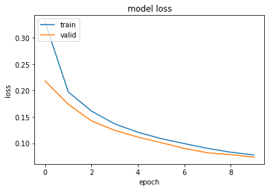
Getting to 96+% validation accuracy in just 4 epochs is quite promising! Interestingly, we observed similar results using 2 or 5 fields, with or without word2vec, and after slightly varying the size of the vocabulary.
Below are the results using the top 1000 vocab words only, with word2vec turned off and using only the first two fields per assembly line (MAX_FIELDS=2). The training progress looks almost identical to the full vocab case, again achieving 97+% accuracy. The model size is much smaller though (~2MB).
 =========================================================================
 Training using Kaggle malware dataset - No word2vec
 MAX_FIELDS = 2 - MAX_SENTS = 5
 MAX_SENT_LENGTH = 20 * MAX_FIELDS = 40
 Vocab size = 1000 unique tokens
 Train on 302877 samples, validate on 33654 samples
 796s - loss: 0.2940 - acc: 0.8792 - val_loss: 0.2103 - val_acc: 0.9242
 809s - loss: 0.1840 - acc: 0.9360 - val_loss: 0.1606 - val_acc: 0.9463
 828s - loss: 0.1508 - acc: 0.9483 - val_loss: 0.1436 - val_acc: 0.9526
 841s - loss: 0.1292 - acc: 0.9568 - val_loss: 0.1196 - val_acc: 0.9603
 862s - loss: 0.1137 - acc: 0.9625 - val_loss: 0.1107 - val_acc: 0.9631
 847s - loss: 0.1018 - acc: 0.9670 - val_loss: 0.0994 - val_acc: 0.9673
 862s - loss: 0.0926 - acc: 0.9701 - val_loss: 0.0949 - val_acc: 0.9695
 854s - loss: 0.0848 - acc: 0.9729 - val_loss: 0.0876 - val_acc: 0.9720
 844s - loss: 0.0787 - acc: 0.9749 - val_loss: 0.0853 - val_acc: 0.9729
 809s - loss: 0.0731 - acc: 0.9769 - val_loss: 0.0771 - val_acc: 0.9759
 =========================================================================
Below are the performance metrics on the held-out 20% test set. We evaluated the test performance per individual sequences, i.e., subsets of assembly code, as well as the overall classification performance per executable using a simple majority vote. Overall accuracy is 97.8% for individual sequences, 98.2% for the programs as a whole.
 =========================================================================
 Sequence Confusion Matrix
 Predicted      0      1  __all__
 Actual
 0          36863    632    37495
 1            854  29885    30739
 __all__    37717  30517    68234
 =========================================================================
 Sequence Performance metrics
 Class 0: Recall = 98.31444193 Precision = 97.73576902
 Class 1: Recall = 97.22177039 Precision = 97.92902317
 Overall Accuracy = 0.9782220007620834    AUC = 0.9776810615749885
 =========================================================================
 Per-executable Confusion Matrix
 Predicted   0    1  __all__
 Actual
 0          82    2       84
 1           2  137      139
 __all__    84  139      223
 =========================================================================
 Per-executable Performance metrics
 Class 0: Recall = 97.61904762 Precision = 97.61904762
 Class 1: Recall = 98.56115108 Precision = 98.56115108
 Overall Accuracy = 0.9820627802690582    AUC = 0.9809009934909216
 =========================================================================
Now compare the same run but using the full vocabulary of 25,573 tokens, with pre-trained word2vec weight initialization. As you see it has produced very close results as compared to the 1,000-token vocabulary without word2vec initialization:
 =========================================================================
 Training using Kaggle_malware dataset - With word2vec
 MAX_FIELDS = 2 - MAX_SENTS = 5
 MAX_SENT_LENGTH = 20 * MAX_FIELDS = 40
 Vocab size = 25573 unique tokens
 968s - loss: 0.2078 - acc: 0.9214 - val_loss: 0.1566 - val_acc: 0.9445
 967s - loss: 0.1365 - acc: 0.9525 - val_loss: 0.1217 - val_acc: 0.9594
 993s - loss: 0.1132 - acc: 0.9617 - val_loss: 0.1109 - val_acc: 0.9620
 953s - loss: 0.0981 - acc: 0.9673 - val_loss: 0.0969 - val_acc: 0.9680
 944s - loss: 0.0877 - acc: 0.9713 - val_loss: 0.0899 - val_acc: 0.9703
 989s - loss: 0.0804 - acc: 0.9743 - val_loss: 0.0790 - val_acc: 0.9740
 1015s - loss: 0.0741 - acc: 0.9761 - val_loss: 0.0795 - val_acc: 0.9741
 1022s - loss: 0.0704 - acc: 0.9773 - val_loss: 0.0709 - val_acc: 0.9777
 1006s - loss: 0.0659 - acc: 0.9788 - val_loss: 0.0718 - val_acc: 0.9769
 1020s - loss: 0.0627 - acc: 0.9797 - val_loss: 0.0657 - val_acc: 0.9788
 =========================================================================
Note that even though the word embedding weights are not initialized, the learned model catches up with the pre-initialized one after one or two epochs.
Finally, these are the performance metrics on the held-out 20% test set: For both sequence and program classification, an accuracy of 98.2% is achieved.
 =========================================================================
 Sequence Confusion Matrix
 Predicted      0      1  __all__
 Actual
 0          37167    328    37495
 1            899  29840    30739
 __all__    38066  30168    68234
 =========================================================================
 Sequence Performance metrics
 Class 0: Recall = 99.12521670 Precision = 97.63831240
 Class 1: Recall = 97.07537656 Precision = 98.91275524
 Overall Accuracy = 0.9820177624058387    AUC = 0.9810029662651356
 =========================================================================
 Per-executable Confusion Matrix
 Predicted   0    1  __all__
 Actual
 0          82    2       84
 1           2  137      139
 __all__    84  139      223
 =========================================================================
 Per-executable Performance metrics
 Class 0: Recall = 97.61904762 Precision = 97.61904762
 Class 1: Recall = 98.56115108 Precision = 98.56115108
 Overall Accuracy = 0.9820627802690582    AUC = 0.9809009934909216
 =========================================================================
Conclusion
Limiting the vocabulary size by normalizing the disassembled content and using the top 1000 unique tokens by frequency in two-field action tuples produces similar performance results as compared to the full vocabulary, with or without word embedding initialization.
Summary
Hierarchical Attention Networks (HANs) are well suited for classification of sequences, leveraging multi-layers of short and long-term memory to capture sequence intent based on context. When applied to malware detection, both statically and dynamically, high detection performance is achieved using a controlled vocabulary size with negligible to no loss in accuracy.
To control the vocabulary size in the training data, several techniques are beneficial:
- Normalization of the raw content to conflate file names, paths, memory addresses, registry keys, etc.
- Considering the most frequent unique tokens only, for e.g., top 1000, captures the most useful signals in the data.
- The first two fields per action tuple, such as (action, target) or (operation, operand), are the most predictive.
The trained model size is proportional to the vocabulary used for training. Model sizes may vary from 2-3 MB with limited vocab up to 80+ MB and more with larger vocab sizes, with similar classification performance.
Resources
- Zichao Yang, Diyi Yang, et al, Hierarchical Attention Networks for Document Classification, HLT-NAACL 2016 (PDF)
- GitHub repository link
- Keras — Python Deep Learning library
- Microsoft Cognitive Toolkit
Cover image photo credit: Photo by Toa Heftiba on Unsplash