Exploring space-time tradeoffs with Azure Quantum Resource Estimator

Ivan Basov

February 28th, 20240 2

Introduction

We are delighted to present a new experience for exploring space-time tradeoffs recently added to the Azure Quantum Resource Estimator. Available both as Azure Quantum Development Kit (VS Code extension) and a Python package, it adds a new dimension to estimates.

Resource estimation doesn’t just yield a single group of numbers (one per objective), but rather multiple points representing tradeoffs between objectives, such as qubit number and runtime. Our recent update of the Azure Quantum Resource Estimator adds methods for finding such tradeoffs for a given quantum algorithm and a given quantum computing stack. We also provide a visual experience to navigate alternatives with an interactive chart and supplementary reports and diagrams:

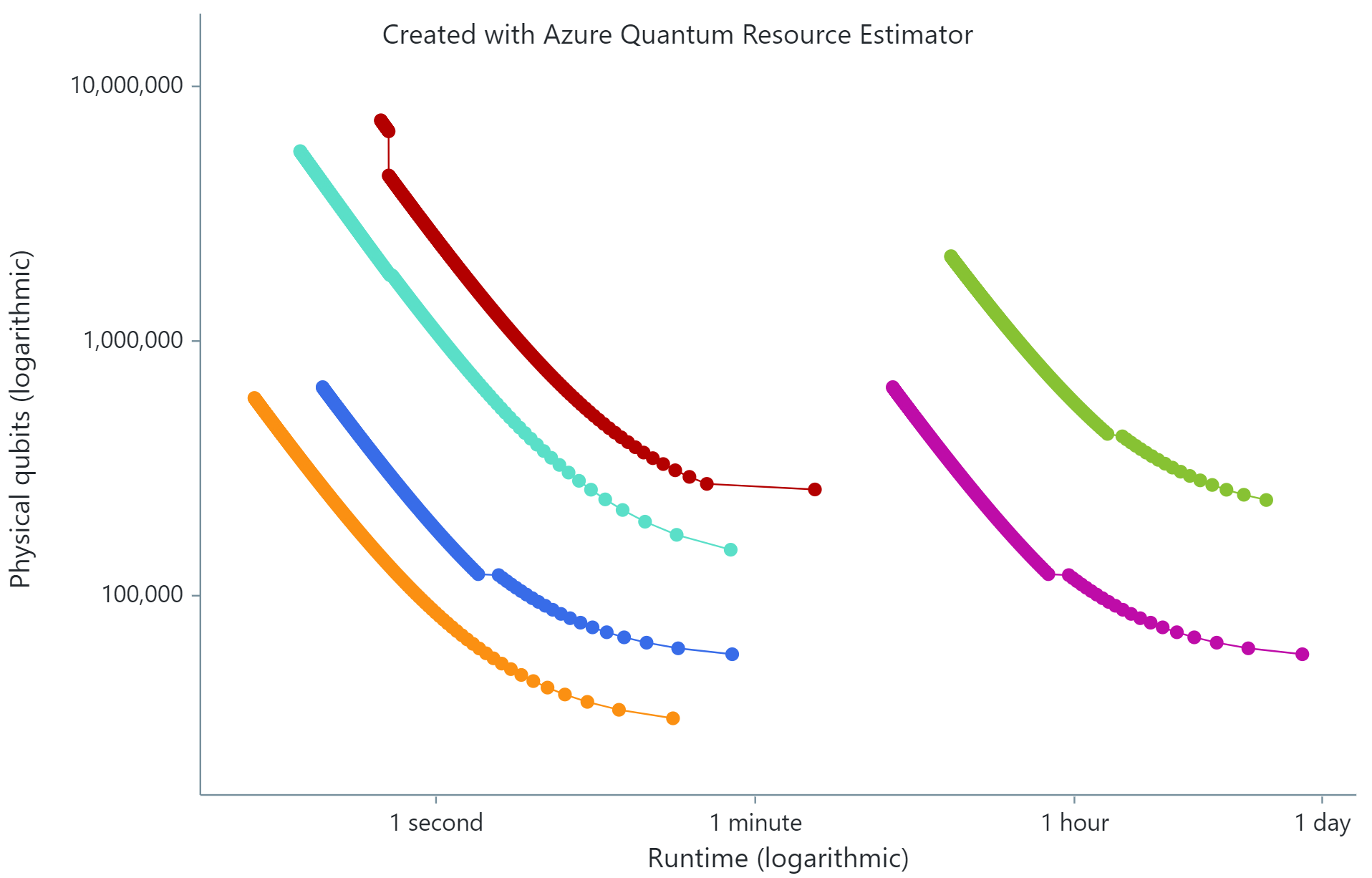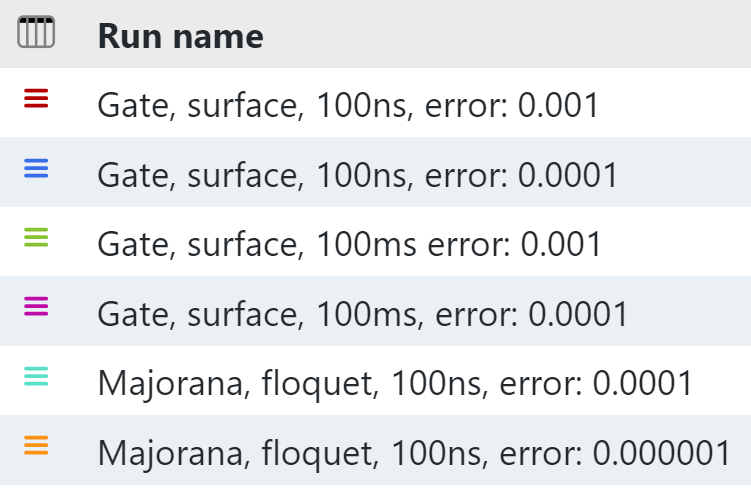
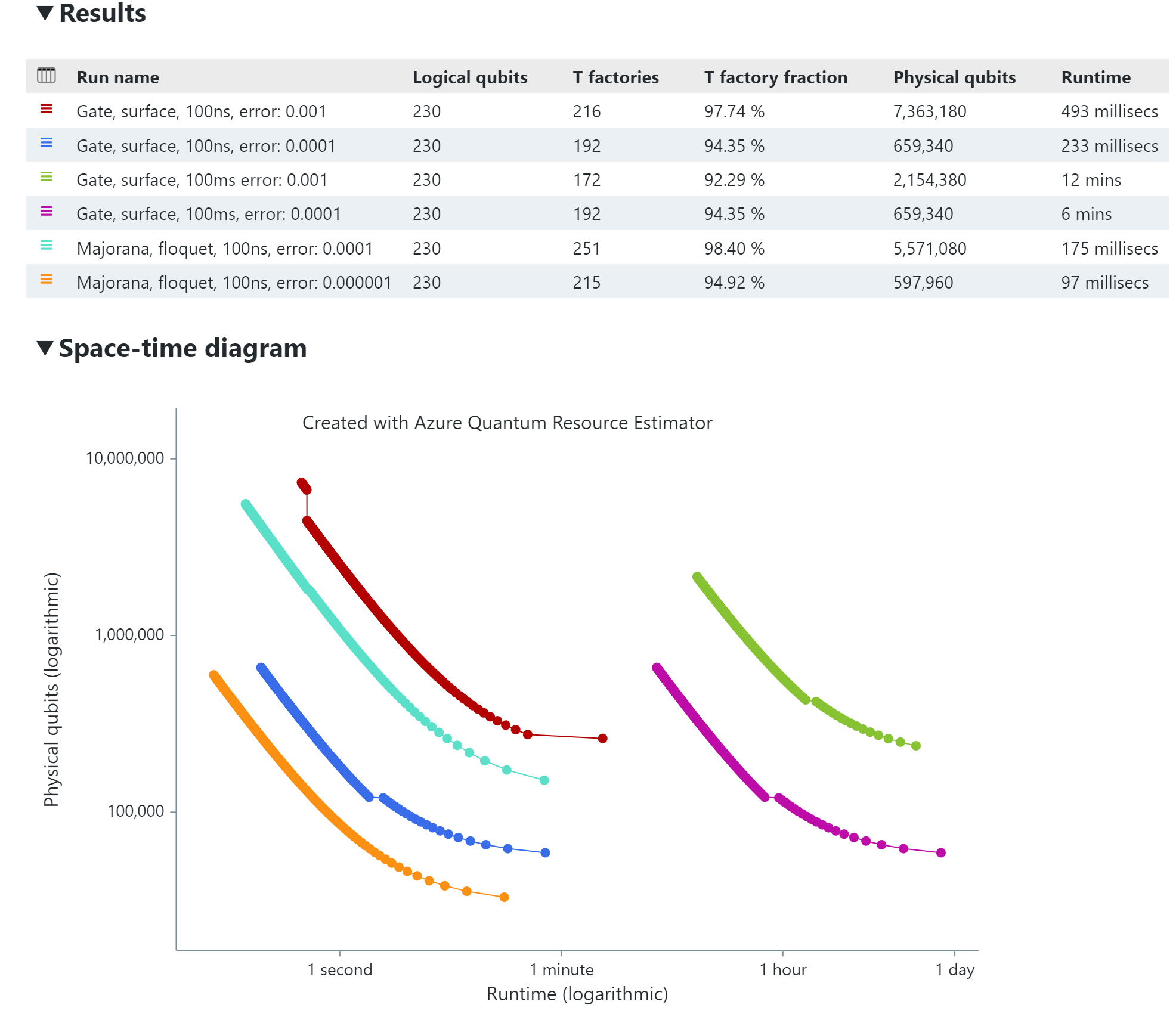
Image Resource Estimator Space-time diagram legend

Image Resource Estimator space time tradeoff diagram

This chart illustrates tradeoffs between qubit numbers and runtimes required for running the same algorithm across multiple projected quantum computers. See estimation-frontier-widgets.ipynb for steps to learn how to generate this diagram.

More specifically, we have considered the simulation of the dynamics of a quantum magnet, the so-called Ising model on a square 10×10 lattice. This is the simplest model for ferromagnetism in a quantum system, and the algorithm simulates its evolution over time. At this system size the problem cannot be simulated on classic computers in reasonable time and solutions with computers would be highly desired.

The diagram above and the table

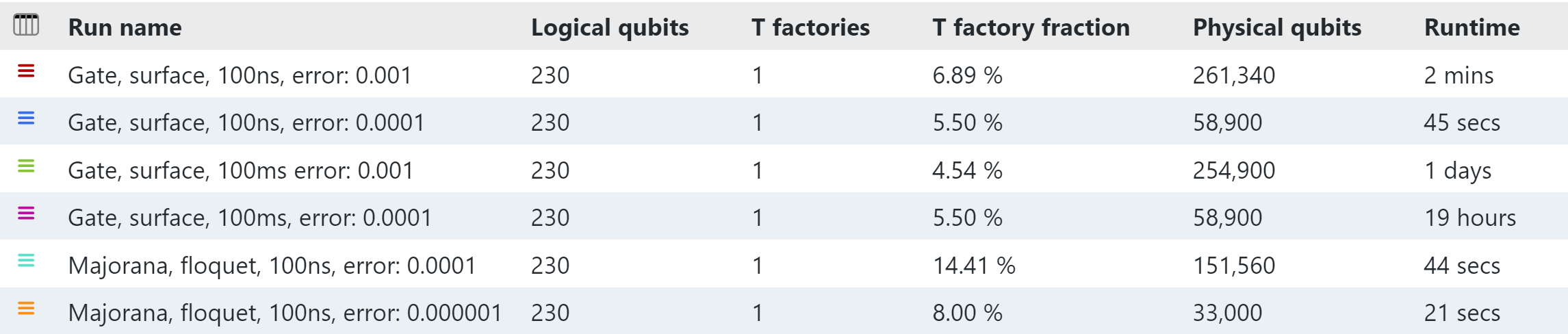
show that this algorithm requires 230 logical qubits with low error rates. Such logical qubits don’t exist yet, and it will require hundreds of noisy physical qubits per each logical. So, the total number of high error rate physical qubits requiring for the simulation ranges from 33,000 to 261,340.

You also can notice on the chart that increasing the number of utilized physical qubits by 10-35 times reduces the runtime 120-250 times. A thoughtful analysis of tradeoffs for entire algorithms and for subroutines can save a lot of runtime if extra qubit resources are available.

Opportunities for space-time tradeoffs

Compromises between the number of physical qubits and the runtime in quantum computations are like ones between space and time utilization in classic computing. As we have done above, for a given algorithm, one can start estimates by computing the minimal number of physical qubits required for its execution on a given quantum stack, and then deduce the corresponding runtime. If more physical qubits are available, one can accelerate the runtime by parallelizing execution of the algorithm or its subroutines.

One can build multiple estimates by allowing more and more physical qubits and improving the runtime. We can consider efficient estimates, such that in each pair of estimates, one would be better than the other with respect to runtime, and the other would be better with respect to the number of physical qubits. The set of such estimates forms the so-called Pareto frontier which is represented by monotonous decreasing plots on the space-time diagram.

Just as in classical programs, there are many opportunities for space-time tradeoffs in the choice of quantum algorithms and their implementation. Here we want to discuss another, quantum-specific opportunity. Rotation gates that rotate logical qubits by arbitrary angles require so-called magic states which are generated in a process known as Magic State Distillation happening in a set of qubits called the “magic state factories”. Many quantum stacks use the T gate as the only magic gate, and corresponding states and factories become T-states and T-factories, and we use those names in the Resource Estimator.

T-state generation subroutines are executed in parallel with the main algorithm. Let us start with a single T-factory. For some algorithms, it could produce enough T-states corresponding for the algorithm consumption. For other algorithms requiring more T-states, the algorithm execution will be slowed down, waiting for the next T-state to be produced. Note that idling of an algorithm is not free in the quantum world because errors in quantum states will occur while waiting. Longer runtimes might thus require a higher error correction code distance and with it more physical qubits and longer runtimes than might naively be estimated.

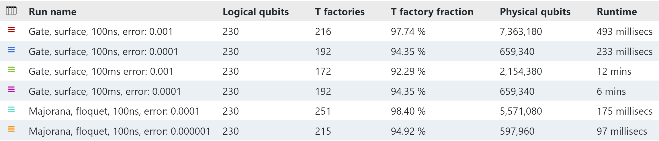
If an algorithm waits for new T-states and there are more qubits available, we can add additional T-factories to produce more T-states. This saves runtime at the cost of more physical qubits. Having enough physical qubits available, we can increase the number of T-factories until they produce enough T-states for algorithm consumption without idling. This will give the shortest runtime of the algorithm. For example, the algorithm considered above could efficiently use up to 172-251 T-factories depending on the computing stack. This involves spending from 92.29% to 98.40% of its resources for T-states distillation.

Building estimate frontiers with Azure Quantum Resource Estimator

As shown in estimation-frontier-widgets.ipynb, to estimate resources required to run a Q# program, one has to run

result = qsharp.estimate(entry_expression, params)

where the “entry_expression” refers to the entry point of the program and params could cover multiple quantum stack configurations and estimation parameters as well.

When “estimateType”: “frontier” is set, the estimator searches for the whole frontier of estimates, otherwise, it looks for the shortest runtime solution only.

Executing the

EstimatesOverview(result)

command visualizes all the estimates found in result (frontier and individual as well) with the space-time diagram and the summary table.

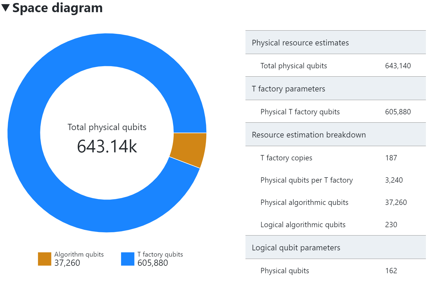
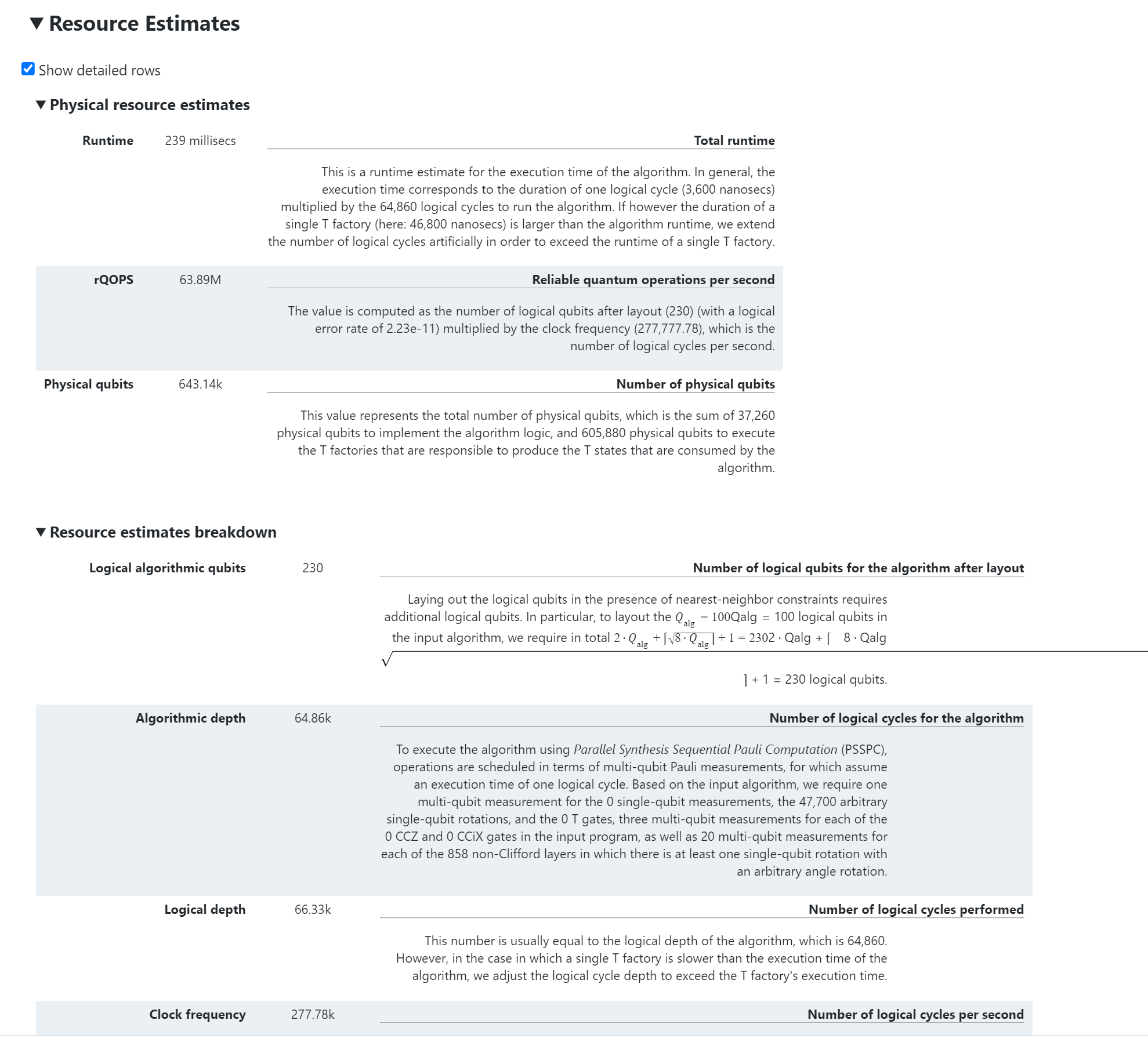
Selecting rows on the summary table or point on the space-time diagram generates the space diagram and the detailed report:

“EstimatesOverview” supports optional parameters for custom color schemes on the space-time diagram and custom series name for the summary table.

More tips and tricks for the “EstimatesOverview” and for supplementary visualization elements are available at estimation-frontier-widgets.ipynb.

Conclusion

Estimating resources for quantum algorithm executions goes beyond providing a single pair of numbers — the runtime and the number of physical qubits. It requires constructing and analyzing the entire frontier of tradeoffs between those objectives. The Azure Quantum Resource Estimator allows you to build and explore those tradeoff frontiers and more accurately evaluate your requirements. With this new data, you can determine if you need to improve your algorithm, develop new error correction codes, or explore alternate qubit technologies.

The Azure Quantum team is committed to continuous improvements in the Resource Estimator. This tool supports both our internal teams and external researchers in the pursuit of designing quantum computers.

Our primary focus is on enhancing the precision of estimates and offering expanded estimation capabilities.

We eagerly welcome your feedback on the specific custom options you require for estimating your quantum computer resources. Your insights will play a vital role in refining our tool, making it even more effective for the entire quantum community.

Learn more about Resource Estimation

Visit our technical documentation for more information on Resource Estimation, including detailed steps to get you started.
Try the sample used for writing the blog post.
Run the Resource Estimator at Azure Quantum Development Kit (VS Code extension). You can try an online version https://aka.ms/qre-demo as well. To estimate a Q# program press CTRL+SHIFT+P and look for “Q# Calculate Resource Estimates” in the drop down menu.