Business Problem
For a subscription service business, there are two ways to drive growth: grow the number of new customers, or increase the lifetime value from the customers that you already have by retaining more of them. Improving customer retention requires the ability to predict which subscribers are likely to cancel (referred to as churn), and to intervene with the right retention offers at the right time. Recently, the use of deep learning algorithms that learn sequential product usage customer behavior to make predictions have begun to offer businesses a more powerful method to pinpoint accounts at risk. This understanding of an account’s churn likelihood allows a company to proactively act to save the most valuable customers before they cancel.
CSE recently partnered with the finance group of Majid Al Futtaim Ventures (MAF), a leading mall, communities, retail and leisure pioneer across the Middle East, Africa and Asia, to design and deploy a machine learning solution to predict attrition within their consumer credit card customer base. MAF sought to use their customer records – including transaction and incident history plus account profile information – to inform a predictive model. Once developed, MAF needed to deploy this model in operation to allow them to make effective retention offers to the customers directly from their customer marketing systems.
Managing churn is fundamental to any service business. The lifetime value of the customer (LTV) is the key measure of business value for a subscription business, with churn as the central input. It’s often calculated as Lifetime Value = margin * (1/monthly churn). Reducing monthly churn in the denominator increases the LTV of the customer base. With increased LTV for the customer base comes increased profitability, and with that increased profit comes the economic support to increase marketing activity and investment in customer acquisition, completing a virtuous cycle for the business.
Technical Problem Statement
Predicting that a customer is likely to churn requires understanding both the patterns in the sequence of user behavior and user state for churners compared to non-churners. Modeling of these user states and behavioral sequences requires using tabular data coming from transaction systems, incident management systems, customer and product records, and then turning these data into a model-friendly set of numerical matrices. This pre-processing of the original tabular data into model-friendly sequences is, in and of itself a significant piece of technical work.
For the prediction task we had to choose whether to predict the attrition event itself or the inactivity that might presage a later attrition. In our modeling approach we predict churn itself. Despite the fact that the actual cancellation decision is a lagging indicator, our model delivered sufficient precision. In future modeling efforts, we will label long-standing inactivity as effective churn.
We worked with MAF to define a performance requirement in terms of accuracy, precision and recall. Once a model performed at the required levels, we could experiment with retention offers for those predicted to cancel. To run these experiments we needed to deploy this predictive model in a secure and operationally reliable environment where we could retrieve batch predictions daily and drive retention offers with the associated workflow.
The Data
The source data includes profile data as well as time series of sequential numerical and categorical information. These data come from historical transaction activity, historical customer incident activity, the product portfolio information and customer profile data. The customer profile data includes state information on the characteristics of the subscriber and the product they are using. The time series of sequential data includes transactions and incidents with a time stamp for each event. In some cases, the time series may have many events in a single day. In other cases, there may be no activity for a period of time.
While we can’t share the anonymized MAF data, we use here three open source examples of source data that is similar in shape and type in order to better illustrate the starting point.
First, we had customer portfolio information, similar to that detailed in the telco churn open data set on Kaggle. These data characterizes the customer demographics, preferences and type of product used. See a selection of the data in the chart below.

Public Data Sample – Customer Profile Data
Next, we have transaction history information. The transaction information used a schema similar to banking transaction information, like that shared in the PKDD 99 Discovery Challenge. See a small snippet of these data in the chart below.

We also had customer incident history. Customer incident data structure the case ID, opened and closed date, category, subcategory and details, as well as status on the case. Below is a sample of a similarly structured data set from a public incident data set from San Francisco on data.gov. You can see that these data track the incident cases, categorization, activity and resolution.

The structure and content of the available data informed our approach for pre-processing and modeling.
Approach
Our project has three parts: pre-processing, modeling, and deployment in operation. We start with pre-processing: manipulating this tabular business application data into the formats that can feed our modeling. This step is highly generalizable to many types of deep learning work with tabular business data.
We broke the data pre-processing work down into several steps. This allowed us to reduce the size of the very large data, especially the transaction tables, for easier manipulation. It also focused next pre-processing steps, enabling our team members to coordinate and focus our individual work more efficiently. And, additionally, it set up the work to be deployed in operation, script by script, into SQL, while allowing us to refine our pre-processing work in later steps as we learned from our early models.
For our sequential modeling approach we required a specific data format. For an attention deep learning model like the Long Short-Term Memory (LSTM) we used, the data need to be expressed ultimately as a three-dimensional array of account x timestep x feature. More details on LSTM data formats are available in this excellent blog post.
Our text information needed to be expressed numerically. We chose to represent the sequence with word tokens, and embeddings. Read more about embedding approaches within this comprehensive blog post.
In our modeling work, we wanted to derive signal from two somewhat different sets of information, the history of incidents and the time series of account-related transactions and states. To do this, we prepared two data sets to supply to a hybrid model. Recent innovative churn prediction models are typically multi-input hybrid models. The first model input is time series numerical data in the account x timestep x feature format that feeds into a bidirectional LSTM. The second model input is textual and categorical incident data to feed a 1D CNN. We used the Keras functional API to easily build a multi-input model. We detail the specific modeling method and choices we made in the section below.
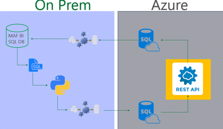
High Level MAF Hybrid Deployment Overview
Lastly, the data pre-processing and the predictive model needed to be deployed into production such that it could be called easily on a per-account basis. For our customer, this required integrating model services with on-premise data, a hybrid cloud and on-premise implementation. The chart here demonstrates how the model will be called in operation. Pre-processed tables are generated in SQL Azure. At a high level, from within an Azure Machine Learning workspace, we retrieve data and then run a model script to generate a prediction score. Then we store the predictions for each account from that batch run into a SQL Azure table for later use by the MAF marketing operations.
The Data Preprocessing
Pre-processing comprises four sequential functional steps with an associated script for each. The first is ‘filtering and formatting’ from the source tables of interest. This reduces the data bulk for our design phase. The second script performs ‘joins, folds and conversions’. It joins our tables of interest, folds the data (sequentially or in aggregate) into our final timestep of interest for our sequential models, and generates meaningful numeric values from non-numeric information. The third script performs feature engineering. In this script we derive additional features and augmented the data in order to provide our models with more signal. We iterated on this script as we refined the model.
We organize these scripts separately so that we could deploy each script individually into SQL for deployment, while leaving us flexibility to iterate on those remaining as we matured our understanding and approach to the model. This approach afforded us speedier collaboration on the later scripts.
The following is an excerpt of the processing done at each stage. To illustrate we highlight just the time series pre-processing and not the text pre-processing. This github repo contains all the pre-processing with more detailed information.
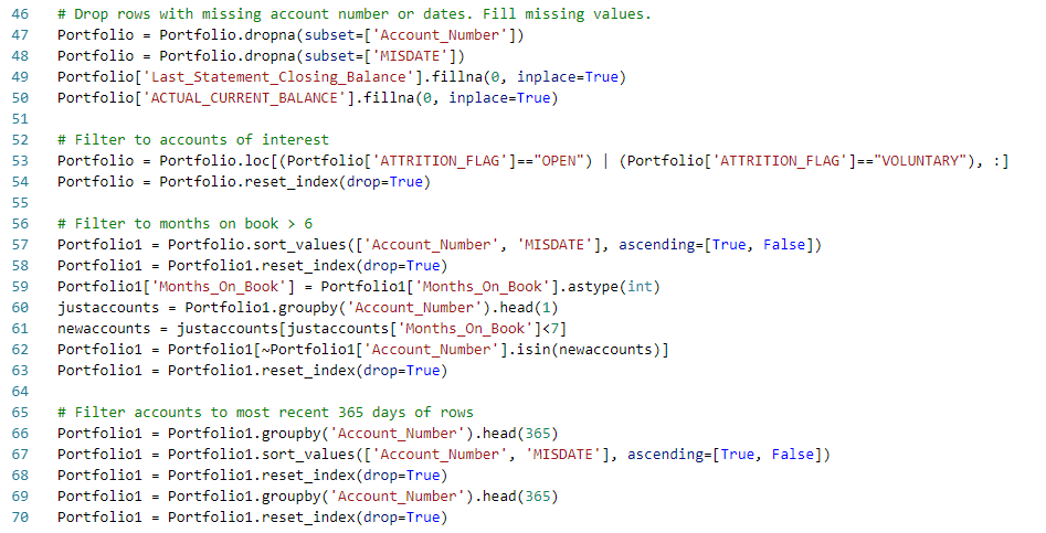
a.) Filtering and Formatting: The goal of this step is to reduce the size of the data passed along to subsequent steps and to do rudimentary formatting and cleaning (e.g. replace missing values and convert datatypes). For example, we selected columns of interest and filtered to eliminate account types that are not in our consideration set. We also limit the history for each account that we bring forward for sampling, reducing the size of the transaction table substantially. With the size of the data reduced, the time required to design the subsequent steps is significantly reduced. A few snippets of the filtering and formatting steps are highlighted below, while the full notebooks are here.
b.) Joins, Folds and Conversions: After filtering the source data, the data are joined to form two data frames. The goal of this step is to get close to having the data in the functional model-ready numerical form, but before much augmentation. This simplifies the later augmentation work.
We chose the ‘daily’ timestep interval to model on. Where the data were more frequent than daily, we ‘folded’ the data – that is, we generated aggregates, concatenations and other descriptive statistics of the information within that day. For example, with the incident data, we concatenated the text descriptions of the incidents of each day, up to the last five. In this iteration, we preserved detail of the last five events that day which captured the lion’s share of the multiple events per day sample. We chose aggregations that expressed the maximums and totals for within day events by type. We also generated conversions of datetime variables, representing them as count-of-day differences (e.g., days since last activity). A selection of steps from this script can be seen here:

c.) Feature engineering: Within the feature engineering step, we removed the predictive period – in our case 14 days – added derivative features, wrote out the final labels, and added new engineered or augmented features to the array or data frame.

Modeling Method
As we noted in the approach section, we applied a multi-input model construction. We used the Keras functional API and combined the textual and categorical data coming from incident history with the time series transaction and state sequence for the account. The multi-input approach allows us to essentially concatenate these and fit the hybrid model.
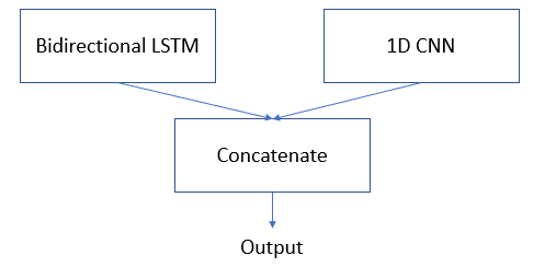
Our sequential non-text information is best harnessed in a Bidirectional LSTM – a type of sequential model described in more detail here and here – that allows the model to learn end-of-sequence and beginning-of-sequence behavior. This maps to domain experts’ knowledge that distinctive behavior at the end of the subscription period presages churn. It also captures the patterns in the progression of events over time that can be used to predict eventual churn.
On the other hand our textual and categorical data need a separate model to learn from this differently structured data. We have several options here. The simplest option that we developed was to convert the sequence of textual and categorical data, coming from our incident data, into a 1D CNN. We created row-wise sequences of textual incident information for each account, tokenized these words, and applied Glove word embeddings for each. These were right-aligned and pre-padded to better learn patterns from most recent dates in order to discern sequences and events that presage churn.
In future iterations, we could add additional input models to learn from non-volatile state and profile information to improve the signal, and categorical embedding modeling for the categorical incident information and other categorical data.
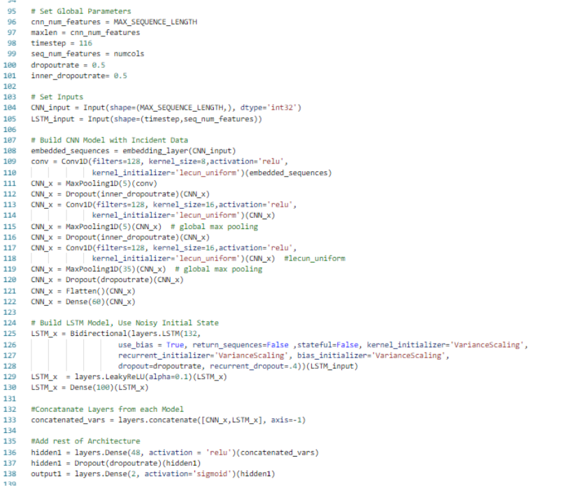
We developed and fit each model input independently to understand its performance. Hyperparameters were adjusted to a good starting point to fit the hybrid model. Then we combined them into a hybrid construction and fit against the two inputs. An excerpt of the model is below, with more about the approach and the rest of the code in this Github repo.
Results
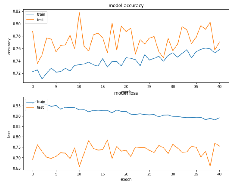
Our multi-input model performed much better at identifying the portion of accounts at risk than either of the independent models. However, while the model can be used to begin to test retention offers and we achieved our performance goal of >80% accuracy, the precision can most likely still be improved with additional data.

Model Deployment
We used Microsoft Azure Machine Learning Service to deploy our model as a REST API endpoint to be consumed/invoked by MAF internal application. Azure Machine Learning service provides the following targets to deploy your trained model:
- Azure Container Instances (ACI)
- Azure Kubernetes Service (AKS)
- Azure IoT Edge
- Field-programmable gate array (FPGA)
We chose Azure Container Instances (ACI) over Azure Kubernetes Service (AKS) as our deployment target for two reasons: First, we needed to quickly deploy and validate the model. Second, the deployed model won’t be used on high-scale as it’s intended to be consumed by just one internal MAF application on a scheduled interval.
To get started with Azure Machine Learning Service and to be able to use it for deploying our model we installed Azure Machine Learning SDK for Python. Azure portal can also be used but we preferred using the SDK to have our deployment workflow documented step by step in Jupyter Notebooks.
As a first step in our deployment workflow we used Azure ML SDK to create the Azure Machine Learning Service Workspace (as shown below). You can look at Azure Machine Learning Workspace as the foundational block in the cloud that you use to experiment, train and deploy your Machine Learning models. In our case it was our one-stop shop for registering, deploying, managing and monitoring our model.

We followed the deployment workflow here to deploy our model as REST API end point:

Scoring File
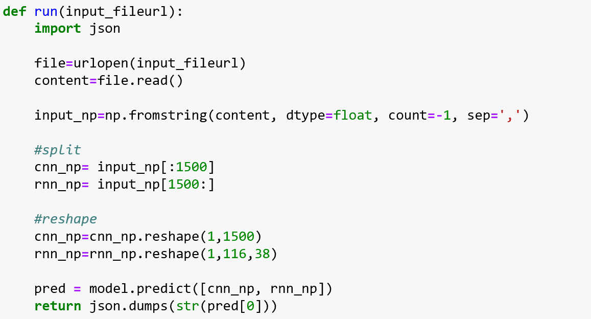
We created a score.py file to load the model, return prediction results and generate a JSON schema that defines our REST API input/output parameters. Since our model is a hybrid model that expects 2 inputs (CNN data and RNN data) we designed our API to take 1 flattened NumPy array that combines CNN and RNN data, which the scorer then splits & reshapes into 2 NumPy arrays: 1D for CNN and 3D for RNN. Once the reshaping is done, the 2 NumPy arrays are passed as arguments to the model for prediction and returning results.


Configuring Docker Image & ACI Container
By having our scoring file up & running, we started working on creating our conda environment file. This file defines our targeted runtime for the Python 3.6.2 model in addition to the dependencies and required packages. For the Azure ML Execution of our model, we needed the following packages:
azureml-defaultsscikit-learnnumpykeras==2.2.4tensorflow
In our Docker image & ACI configuration step, we relied on azureml.core to configure our Docker image using the score.py and conda environment.yml file that we created. Additionally, we configured our container to have 1 CPU core and 1 gigabyte of RAM, which is sufficient for our model.

Register the Model, Create the Docker Image, and Deploy!
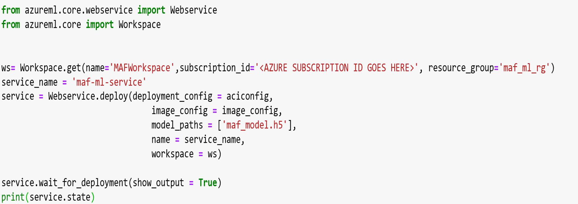
In our final deployment step, we used Webservice.deploy() method from Azure ML Python SDK. This enabled us to pass our model file, Docker image configuration, ACI configuration, and our created Azure ML Workspace to perform each of these steps for every new model we deployed:
- Register the model in a registry hosted in our Azure Machine Learning Service workspace.
- Create and register our docker image. This image pairs a model with a scoring script and dependencies in a portable container, taking into consideration the image configuration we created. The registered image is stored in Azure Container Registry.
- Deploy our image to ACI as a web service (REST API). We deployed the model directly from the model file. This option registered the model in our Azure Machine Learning Service workspace with the least amount of code; however, it allowed us the least amount of control over the naming of the provisioned components. The other way of doing it is to use Model. Register() method first to control the naming of your provisioned resources.
Once the deployment is fully executed, we were able to visualize the resources provisioned in addition to the registered model, image created and web service through Azure portal.
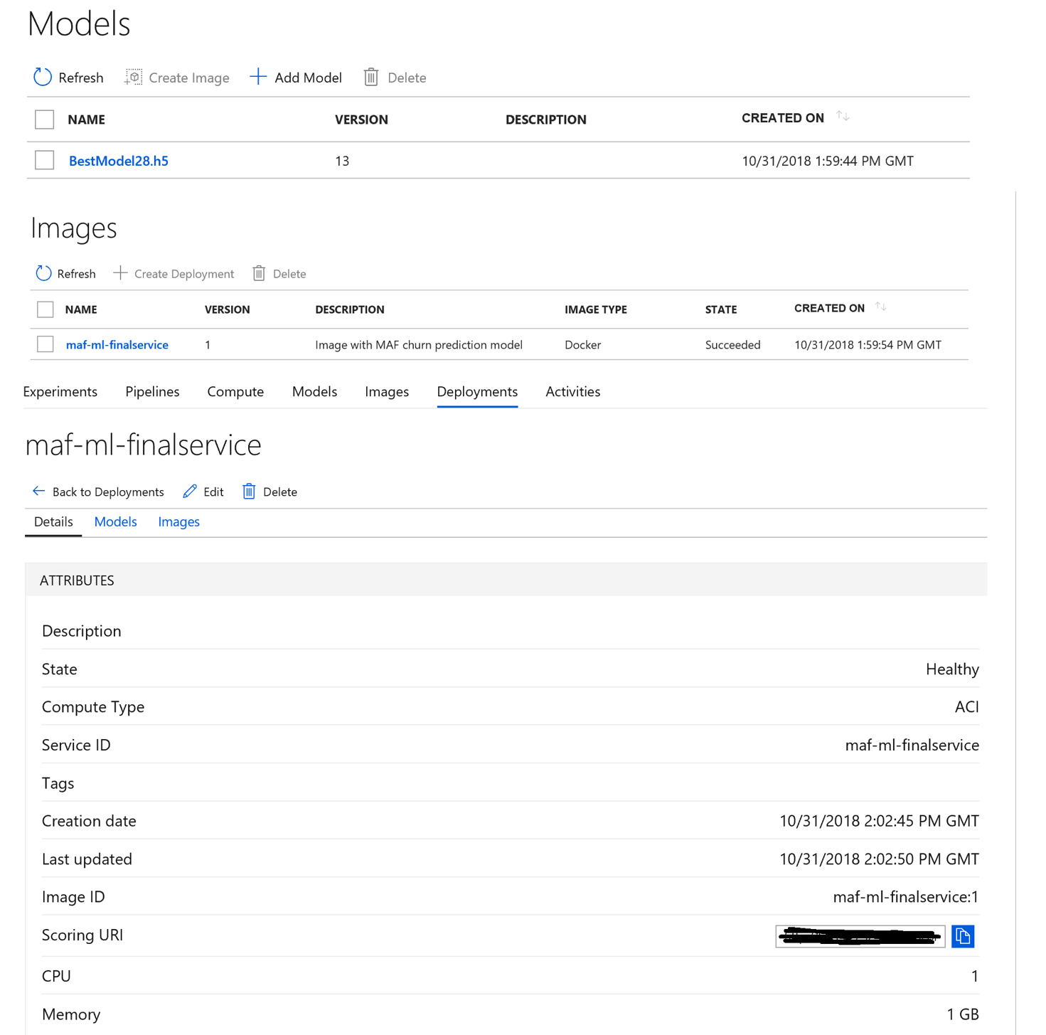
Figure 5: Azure Portal Deployment Screenshots
Conclusion
We have shared an end-to-end example of preparing tabular business data, combining hybrid data to generate sequences that can be used to train a multi-input deep learning model. We have also shown how to deploy the model in operation using Azure ML Workspace and services and Azure Container Instances.
MAF now has an initial model that they can use in operation to identify likely churners and take proactive action to retain these customers. The AML Workspace and ACI environment will allow MAF to continue to update this model. For example, the model accuracy may be improved by adding additional data sources and more transaction details beyond our simple daily aggregates. They can also run additional models within the same environment for other purposes.
We hope that this blog is of use to others building prediction models of a combination of transaction and account information. You can find the code and scripts we developed for data pre-processing here, for modeling here, and for the deployment here. Please feel free to reach out if you have any questions.
