
We’ve been discussing the commit-graph feature in Git 2.18 and how we can use generation numbers to accelerate commit walks. One area where we can get significant speedup is when presenting output in topological order. This allows us to walk a much smaller list of commits than before. One place where this breaks down is when we apply a filter to our results.
For instance, if we filter by a path, then we are asking for a set of commits that modified that path. The following Git command returns the commits that changed “The/Path/To/My/File.txt” in the master branch:
git log master -- The/Path/To/My/File.txtIf the path is not modified very often, then we need to walk more of the commit graph in order to return the results. What’s more, we need to walk a number of trees to determine if the path was modified. In the example above, we need to walk five trees: the root tree and four nested trees for the directories above “File.txt”.
These behaviors combine to make some history calls slow. But in Visual Studio Team Services (VSTS) we speed up file history calls using some powerful tech: Bloom filters.
Today, I’ll describe how we use Bloom filters to accelerate file history calls in VSTS and how we plan to extend the commit-graph feature in Git to use them, too.
File History in Git
Before we get into the details of Bloom filters, we first need to describe how file history works in Git.
Each commit in Git points to a complete description of the working directory at that point in time. In this way, Git is a Merkle tree. Files are represented by blobs, and directories are represented by trees (which reference blobs and other trees), and commits reference their parent commits and their root tree object. A diagram below shows a simple repo with three commits and a few trees and blobs.
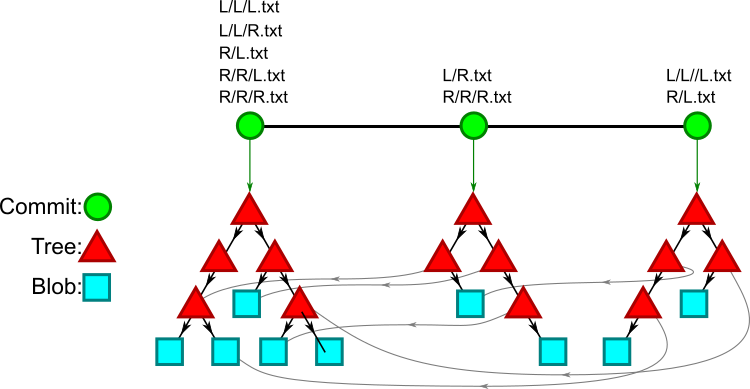
Listed above the commits are the paths that are added or modified by that commit. Note that trees and blobs are shared between commits if they have the same contents. This is the critical ability of the Git object database to have each commit store a snapshot of the entire working directory without storage growing out of control. This also means that when we are performing a checkout or file history operation, we are walking the object graph, a supergraph of the commit graph.
This makes Git very fast when you want to do a git checkout, but can make file history more difficult. In order to determine if a commit “modified” a path, we actually need to determine if that path is different from the path in a parent. To compare a path between two commits, we need to walk two lists of tree objects, parsing each one before finding the next. This is more expensive the deeper the path.
This is further complicated in that Git uses file history simplification by default, and the most important condition is whether the first parent is different. If a path is the same on the first-parent, then we say the commit did not modify the path and we only walk to the first-parent. This is very important to our discussion below, so I recommend you read this article about file history simplification if you want to follow along in full detail.
This computation to determine if a path is different between a commit and a parent is very expensive, especially as the number of subfolders increases. Each folder in the path is another tree that needs to be found, parsed, and examined. We can short-circuit if two trees at the same level of the path are equal, but if our full path doesn’t change very often and a sibling path does change often, that is not enough to help us.
For example, suppose we are performing file history for a path /The/Path/To/My/File.txt. The animation below shows a line of eight commits and the chains of trees that we need to walk as we check each commit to see if it changed the blob at that path. Only three commits fit our file history filter, as they have a different blob at that path than their parent; the last commit is a root commit containing the path, so it is an “add”.
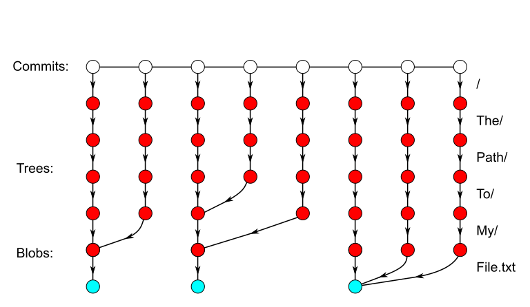
Instead of walking these trees, we would like to have an oracle that can tell us “These two commits have the same content at this path” or “These two commits have different content at this path”. One such oracle could be a list of all commit-path pairs where that path changed at that commit, and we could look up each commit-path pair for our path.
That solution requires a lot of space. There was a point in time where VSTS stored that list in SQL and that table was over 60 GB just for the Linux kernel repository. That’s more than the data you get when you clone that repo! (We have since deleted the table, since we don’t need it anymore!)
Instead, we will settle for an oracle that can provide these two answers:
- This path is the same between this commit and its first parent.
- This path is probably different between this commit and its first parent.
The “probably” in that second answer is the reason we can use Bloom filters to implement this oracle. If we get a “probably” then we can compare the two commits and find out the real answer. We normally did that work anyway, but now we will skip comparing the commits if we get the first answer. In the figure above, the light-colored trees are objects we could avoid walking if we had an oracle like this one (and it was always right). In real-world repos, the density of “skippable” trees is much higher than in this toy example.
We’ll talk about the full application, but first let’s learn about Bloom filters.
What is a Bloom filter?
A Bloom filter is a probabilistic set. To use one, we create a memory region of a certain size (relative to the expected number of elements), then “add” elements to the set by flipping some bits in that region to “on”. We then ask the set
A regular set would provide two answers: “yes” or “no”. A probabilistic set relaxes these answers by allowing “maybe”. For a Bloom filter, we specifically allow the following responses:
- X is definitely not in the set.
- X is probably in the set.
The power of a Bloom filter is that we can avoid doing some hard work when we get the answer “definitely not”. To be correct, we need to check — using other means — that the “probably” answer is actually “yes”, but if we’ve done it right the false positives are very rare.
To create a Bloom filter, we need two magic constants. Recommended values of these constants are 10 and 7, so I’ll just use the concrete numbers instead of constants. These numbers roughly correspond to the size and density of the filter.
Size: If we expect the Bloom filter to contain N elements, reserve at least 10N bits. These bits all start in the “off” position.
Density: For each element X we add to the filter, we will set 7 bits to the “on” position. We will use seven hash values based on X to determine these positions. Turns out that we don’t need seven independent hash functions but instead can combine two mostly-independent hash functions (such as the .NET hashcode and Murmur3) and combine them into an arbitrary number of hash values.
Here is where the magic happens. To check if the Bloom filter contains an element, we see if the 7 bits corresponding to the 7 hash values are on. If any are missing, then we definitely did not add that element. If they are all on, then we probably added that element, but it is possible that we had enough hash collisions that this is a false positive. The trick is setting the magic constants to balance the expected false positive rate with the storage cost. The values 10 and 7 give roughly a 1% false-positive rate.
In the animation below, we create a Bloom filter and fill it with three elements, x1, x2, and x3.

After adding the elements, we then test that x1, x2, and x3 are in the set, which succeeds. We then test elements y1 and y2. The first, y1, is not in the set as it is missing a bit for one of the hash values. However, y2 reports being in the set. Since the image is colored, we can see that the bits were set by different additions, but we only store single bits. Thus, we must say that y2 is probably in the set.
With the magic constants, we expect less than 7/10 of the bits being on (we expect some collisions when adding the elements). If the hash algorithms are sufficiently distributed, then we expect a probability less than 7/10 that any single hash value has its bit on. To have all seven values on then multiplies across this probability. For a full description of how to calculate a false-positive rate, go read a paper on it. Whatever values you use in your implementation, it may be good to generate random inputs and measure the false-positive rate yourself.
How does a Bloom filter help with file history?
For each commit, we can compute the list of paths that change relative to the first parent of that commit. For single-parent commits, this is usually the changes introduced by a single developer in a small unit of time. For merge commits, this is usually the list of changes introduced by a pull request. Remember: if a file changed, then every parent folder also changed.
If the number of changed paths is not too large (we use 512 as a limit in VSTS) then create a Bloom filter and seed it with the values for those paths. If there are more than 512 changes, then we mark the commit as “Bloom filter too large” and check every path. We selected this limit after finding the number of changes in a commit against its first parent roughly follows a log-normal distribution and commits with more than 512 changes are very rare. These commits are usually large, automated refactoring changes that affect most paths in the repository.
In the animation below, we repeat the file history query from the previous animation. This time, we have Bloom filters for the changed paths at each commit. If the Bloom filter returns with “definitely not”, then we do not need to walk trees to check if the commits have the same file at that path. Otherwise, we walk trees to check equality. In one case, the Bloom filter provides a false positive.
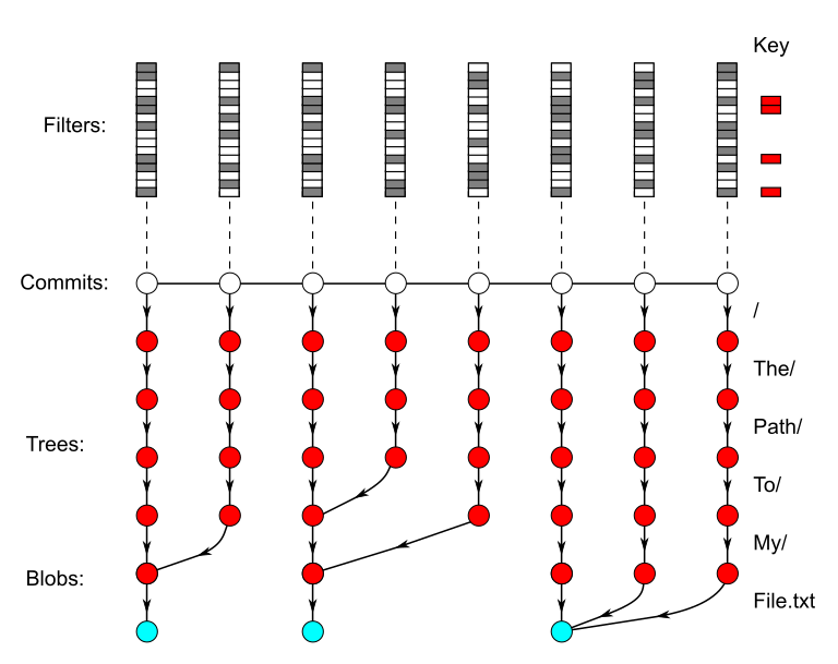
In reality, there are many more “same” commits than “edit” commits for deep paths, so the filters save a lot more walking than in this small example.
With a false-positive rate of 1%, this means that we can theoretically speed up our file history algorithm by 100x by avoiding 99% of the computation. In reality this is closer to a 6x speedup for a random sample of paths. However, we have observed speedups as high as 20x for rarely-changed paths, which was the main application of this effort. The best part is that this requires less than 100MB of extra storage for a repository the size of the Linux kernel.
I personally believe this application of Bloom filters is quite novel, since we are testing one “key” against many small filters. Normal applications check many keys against a single, very large filter.
What does this mean for Git?
The Bloom filter feature already exists on the VSTS Git server, helping file history questions since November 2016. Our goal now is to deliver this for all Git customers!
Earlier, we discussed the commit-graph file format. This file is organized into a list of “chunks”, sorted by a table of contents at the beginning of the file. We can add an optional Bloom filter chunk, so users who want to do some extra computation during Git maintenance can create a commit-graph file containing this Bloom filter information. We could also send the commit-graph file as a new verb in Git Protocol V2. We discussed this addition to the file format and protocol at the Git Merge 2018 contributor’s summit and on the Git mailing list.
Work to implement the feature is planned, so keep an eye out for it in a future version of Git!
0 comments