Scaling IoT/Time Series/Metering Workloads with Azure Cosmos DB for PostgreSQL

Introduction :

For many organizations around the world, the capture of consumption data is a common yet critical requirement. Some of these organizations struggle to manage the sheer volumes of data that they must capture and process. No wonder! We conservatively estimate that there would petabytes of such data globally and it is likely growing at a rapid rate.

Today, many of the systems tasked to handle this data were designed decades ago, and many are likely hosted ‘on-premises’. We have seen, firsthand, such systems can be incredibly difficult to scale, costly to operate and complex to maintain. This all has the potential to simultaneously increase business risk and limit business growth.

Two of the most common industries where we see large scale consumption data workloads are;

• Telecommunications : Voice and Data usage
• Utilities : Energy or resource consumption such as electricity, gas or water

In these industries, once the data has been captured it is often used for a variety of business purposes including;

1. Revenue Collection or Billing
2. Analysis e.g. Seasonal Trends, Demand Forecasting, Peak periods etc.
3. Reporting e.g. Ad-hoc Customer Enquiries, Supporting dispute resolution etc.
4. Auditing and compliance

What is often downstream of this data is a billing system of some description that is used to transform this data into customer invoices or statements. It is quite often the case that in addition to the billing system there is also an analytics system.

While the subject of this blog is specific to the Energy/Electricity industry, the technology we will showcase is equally capable of handling workloads across many industries, including Healthcare, Manufacturing, Monitoring, FSI and others.

If you want to see how we helped a number of Energy industry companies modernize their data platforms to provide performance, scalability and simplified data management for these ever-growing datasets then please read on.

What is Azure Cosmos DB for PostgreSQL :

Even today we often hear “relational databases can’t scale” and “you can’t run OLTP and Analytics on the same database” …. whilst those statements may have come from an era where CPUs were few and storage was painfully slow, today with Azure Cosmos DB for PostgreSQL service those statements no longer hold true.

Azure Cosmos DB for PostgreSQL is a fully managed Azure Database as a Service (DBaaS) where you leave the heavy lifting to us and focus on Applications and Data. More details are in the following link Introduction/Overview – Azure Cosmos DB for PostgreSQL but here is a summary;

• Is built with Open Source PostgreSQL and is powered by the Open Source Citus extension
• Scales to 1000s of vCores and Petabytes of data for a single PostgreSQL ‘cluster’ that can handle the most of demanding of workloads
• Is ideal for a number of uses cases such as high throughput transactional, real-time analytics, multi-tenant SaaS and others

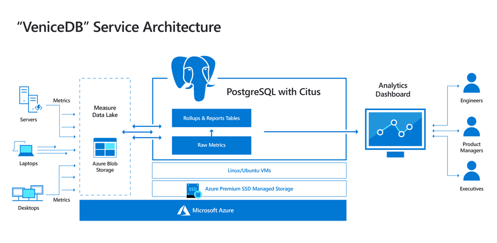
We have seen some great articles showcasing the power of this offering when it comes to large scale data requirements such as Petabyte scale analytics and IoT. In particular, these two blogs explain how we Architected petabyte-scale analytics internally at Microsoft;

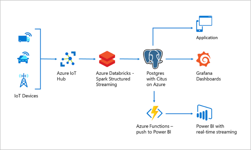
and how building IoT applications with Azure Cosmos DB for PostgreSQL, formerly Hyperscale(Citus) Building IoT apps using Postgres, Citus, and Azure is a popular choice given the data involved and the typical volumes;

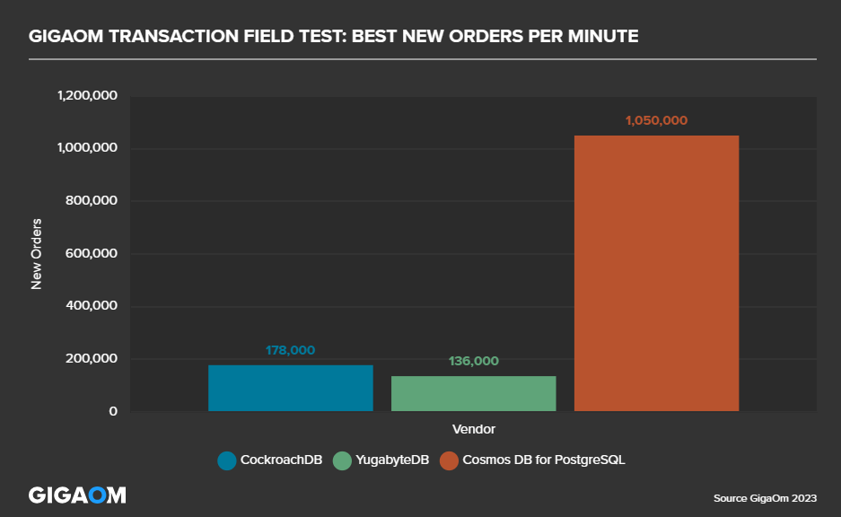
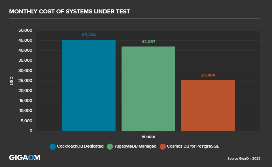
In terms of benchmarks, Azure Cosmos DB for PostgreSQL is capable of some very impressive performance. We have seen that it also costs significantly less than other distributed PostgreSQL offerings. The full details are here Distributed PostgreSQL benchmarks using HammerDB, by GigaOM – Azure Cosmos DB Blog (microsoft.com), but to summarize, it was able to perform many times better than the competition at a fraction of the cost;

Hopefully you are hanging in there, and you can see that we have a service that is capable of amazing performance, scale and cost effectiveness.

Background:

Billing data is considered business critical by most organisations, as it is the final step in revenue realization. It makes sense that the data that was used to generate the billing information should also be categorized as such. This is where the concept of ‘Single Source of Truth’ is often heard and this data is typically stored in a transactional database given its criticality.

In the Australian Electricity Market, metering data is mainly distributed as CSV files and the format of those files is specified by the Australian Energy Market Operator (AEMO). The format specification is called ‘NEM12’ and is in a structured format. Here is a snippet of such a file. Notice that ‘300’ Lines ‘Interval Data Record’ are readings for the given day;

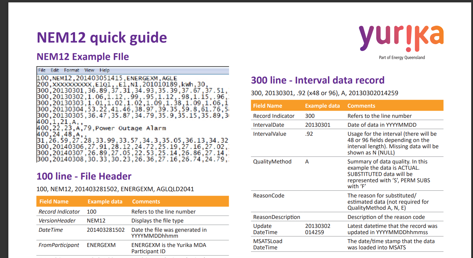
The above screenshot was taken from this document NEM12 Fact Sheet (yurika.com.au). For a more detailed understanding of the file format, you can checkout this document Meter data file format specification nem12 & nem13 (aemo.com.au).

What typically happens is that this data is read from these CSV files, often by some sort of scripting language such as python, and uploaded to a database for storage and further processing. Many organisations rely on this metering data daily. For example, retailers, distributors and generators often store this data in a relational database, often MS SQL or Oracle. This ‘metering‘ database is typically seen as the ‘Single Source of Truth’ for this data and as such it often underpins most billing systems and downstream revenue processes.

This type of metering data is not strictly IoT or Time Series, but almost a hybrid of the two. As we will see throughout this article, Azure Cosmos DB for PostgreSQL has some pretty compelling features that make operations and management of this data very straightforward.

One of the key requirements of metering data in this context is that often there can be data that is ‘restated’, which basically means, that it can be updated over time. For example, it is possible that an attempt to read a meter fails for any one of a variety of reasons, such as a communication error. In this situation it is common that ‘Substitute’ data is provided instead. After some time, the meter will eventually be read and the ‘Actual’ data will be supplied. There are 2 likely options to handle any data updates;

1. 1. Modify the records in the database for the updated data
   2. Insert the updated records and handle the “duplicates” in the application or through database management tasks such as stored procedures

Typical requirements for such metering systems are;

• • Scalable ingestion
  • Low latency ad-hoc queries
  • Analytics such as aggregations
  • Individual meter reporting

Azure Cosmos DB for PostgreSQL to the Rescue:

Back to our ‘NEM12’ data. I have created the following standard PostgreSQL table as an example of one way to store it;

create table meter_data (

nmi varchar(10) not null,

uom varchar(5) not null,

interval_date date not null,

interval_val numeric[],

quality varchar(3) not null,

nmi_num bigint not null,

update_datetime timestamp not null,

primary key (nmi, interval_date, quality, update_datetime)

) partition by range (interval_date);

Table details;

• • ‘nmi’ is the meter device ID.
  • ‘interval_val’ is a native PostgreSQL numeric array type, which caters for any number of values such as 30 minute intervals (48 values) or 5 minutes intervals (288 values) without the need to modify the table structure to cater for a changing number of intervals.
  • The primary key includes the ‘update_datetime’ column to support ‘restated’ data for an already existing ‘nmi’ and ‘interval_date’.
  • PostgreSQL native partitioning has been used to partition the underlying table by ‘interval_date’ on a monthly basis
  • It is also an option to store the interval values as individual rows but that would lead to significantly more rows in your database for no real gain and perhaps an increased management overhead

With this standard PostgreSQL table, we can also make use of the Azure Cosmos DB for PostgreSQL User Defined Function (UDF) to simplify partition creation. Here is an example of a call to the UDF ‘create_time_partitions’ https://learn.microsoft.com/azure/cosmos-db/postgresql/reference-functions#create_time_partitions that creates monthly partitions on the meter_data table from 2010 to the end of 2023;

SELECT create_time_partitions(table_name:= ‘meter_data’,

partition_interval:= ‘1 month’,

end_at:= ‘2023-12-31’,

start_from:= ‘2010-01-01’);

In addition, PostgreSQL with the open source ‘Citus’ extension provides PostgreSQL with the super-power of distributed tables. It can be used to further split, or ‘shard’ your data across multiple compute nodes. For example, with a 4 node cluster, if you run this command to ‘shard’ your meter_data table by the ‘nmi’ column;

select create_distributed_table(‘meter_data’, ‘nmi’);

You would end up with something like this;

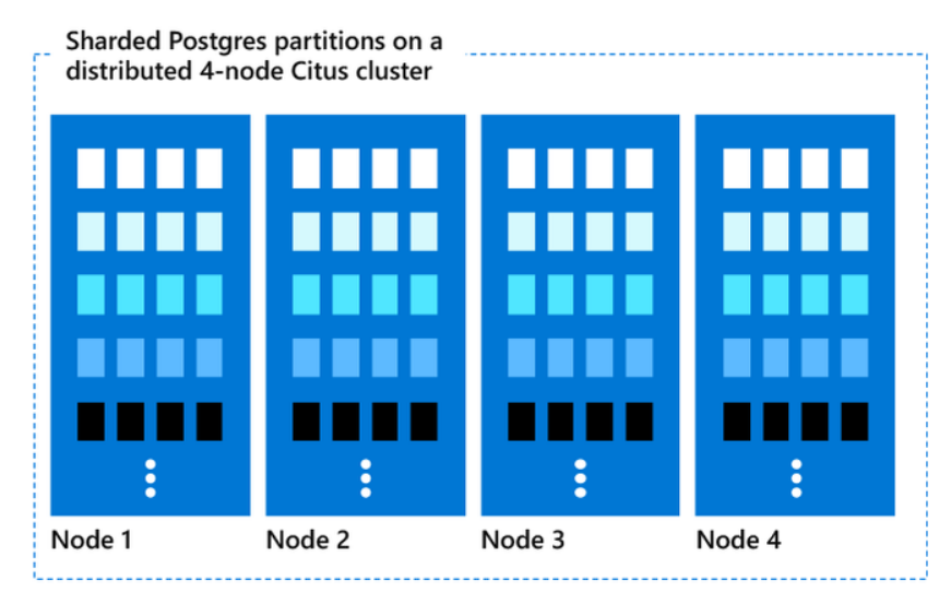
Not only have we partitioned by ‘interval_date’ we have also ‘sharded’ by ‘nmi’. And our meter_data table is now spread across 4 nodes. Each of these nodes has their own compute and storage and can operate independently of the other nodes in the cluster. Here is a link to a great article detailing the similarities and differences between partitioning and sharding in PostgreSQL Understanding partitioning and sharding in Postgres and Citus – Microsoft Community Hub

It is possible to have 100s of nodes in a cluster allowing for truly massive scale to handle the largest of relational datasets and workloads. Amazingly, your application does not even have to know that your table has been sharded across multiple nodes. You still use standard PostgreSQL SQL commands and if they filter on the shard column, ‘nmi’ in this example, then they will be directed to the nodes that hold the required data. Once the node receives the query, it will have all the power of partitioning. All you have to do is run the ‘create_distributed_table’ UDF and the sharding is applied automatically as show in this illustration;

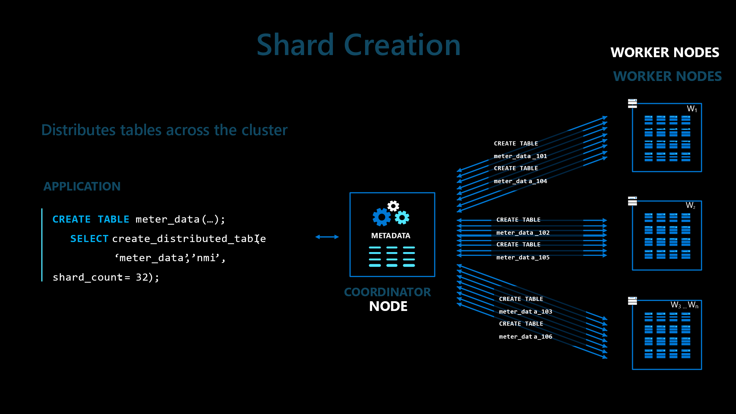
The co-ordinator node of the cluster stores metadata that identifies which distribution column ranges are stored on which underlying worker node. As you can see, the transparent sharding and partitioning of tables across multiple cluster nodes sets your database up to take advantage of parallelism.

Ingestion Scalability:

To demonstrate the scalability of the service, we created and ingested a small dataset into the meter_data table. We have 47GB of ‘NEM12’ like CSV files that consists of 10000 unique NMI with 10 years of daily data (5 minute intervals with 288 interval values per day). The resultant PostgreSQL table size is 46GB and contains 36.52 million rows (10,000 * 3652).

What we are about to illustrate here is an example of one approach where files are ingested into the database in a batch fashion, however, there are many alternate approaches that could be considered such as Real-time data ingestion with Azure Stream Analytics – Azure Cosmos DB for PostgreSQL | Microsoft Learn.

For the tests below, the psql command was run from an Azure VM in the same Australia East region as the database server itself. Specs for the VM were as follows;

• • Standard D16as v5
  • 16 vcpus
  • 64GiB RAM
  • 1TB SSD with max 5000 IOPS

Data was loaded in a multi-threaded fashion using the Linux command line and the PostgreSQL \COPY instruction (PostgreSQL: Documentation: 16: COPY) via the standard PostgreSQL ‘psql’ utility;

find . -type f | time xargs -n1 -P32 sh -c “psql -U citus -c \”\\copy demo.meter_data from ‘\$0’ with csv\””;

The following table shows 4 tests, each with a different cluster configuration, and the time taken to load the dataset;

Test	Co-Ordinator vCores	# Worker Nodes	Worker Node vCores	Worker Node Storage	Total Cluster vCores	Threads	Load Time MM:SS	TPS
1	32	4	4	2TB	48	32	5:52	103k
2	96	8	4	16TB	128	96	2:21	259k
3	64	8	16	16TB	192	64	1:35	384k
4	96	8	8	16TB	160	96	1:21	450k

 

The fastest was test #4, which is interesting as it didn’t have the most total cluster compute at 160 vCores. Test #3 has 192 total vCores but was beaten by the more appropriately configured test #4 as it had more co-ordinator compute, and in these ingest heavy scenarios, co-ordinator compute resources can sometimes affect ingestion throughput more than worker node compute resources.

They key things to highlight with the tests are;

• • 16 vcpus/vcores on the client could be a bottleneck where the thread count increases
  • From 100k TPS for a relatively small cluster up to 450k TPS for a still moderately sized cluster is very impressive for a relational database, rivalling some NoSQL databases, and with the beauty of ANSI SQL support, ACID compliance, referential integrity, primary keys and joins !
  • We used an 8 node cluster in most of our tests, bear in mind 20 nodes are available through the portal and it is possible to request even more than 20 nodes by raising a support request.
  • There are many ways to configure a cluster for optimal performance, whether your workload is write heavy, read heavy or perhaps somewhere in the middle with an even split between reads and writes. You are free to choose any permutation to cater for IO or CPU intensive workloads.

As a side note, what we saw in our test above was that the co-ordinator node could be a bottleneck with an ingest heavy workload. To alleviate this, it is possible to use a special feature that makes it possible to spread an ingest heavy workload directly across all worker nodes (bypassing the co-ordinator if necessary) to essentially bypass any co-ordinator bottleneck. Every node in the cluster has an up-to-date copy of the cluster metadata, and by extension, knows what data lives on which worker node. The details are available here Citus 11 for Postgres goes fully open source, with query from any node (citusdata.com) but hopefully the following picture “paints a thousand words”;

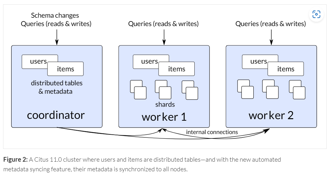
Note that COPY and any DML is supported, including INSERT, UPDATE, DELETE and of course SELECT. Making Azure Cosmos DB for PostgreSQL a scalable solution not just for reads but also for writes, which is unlike many cloud services where you can typically only scale your database for reads.

Query Performance:

Now that we have demonstrated the ability to scale ingestion, we will move on to querying the data. For the purposes of this test, I have used a dataset with 2.5x more data. This larger dataset consists of 25000 NMI with 10 years of daily data. The table size is now 116GB and contains ~91 million rows (25,000 * 3652).

We will run four queries as part of these tests.

Query	Description	Notes
1	Aggregate of the entire table using ‘count’	Scans the entire table
2	Aggregate of the entire table using ‘sum’	Scans the entire table
3	Aggregate 2 columns for 10 random NMI	Using random to avoid caching
4	Monthly rollup using latest interval_date data	Manages ‘duplicate’ data for ‘restated’ intervals

Here are the actual queries used;

Query 1

select count(1) from meter_data

Query 2

select sum(nmi_num) from meter_data

Query 3

select nmi, date_trunc(‘month’, interval_date) as ym , sum(nmi_num), avg(nmi_num)

from meter_data

where nmi in (select nmi from meter_data order by random() limit 10)

group by nmi, ym

order by nmi, ym

Query 4

select nmi,

date_trunc(‘month’, interval_date) AS year_month,

sum(single_val) AS aggregated_value,

current_timestamp AS update_datetime

from (

select distinct on (nmi, interval_date)

nmi,

interval_date,

unnest(interval_val) AS single_val

from

meter_data

where

nmi in (select distinct nmi from meter_data)

and

interval_date between ‘2023-09-01’ and ‘2023-09-30’

order by

nmi, interval_date DESC, update_datetime DESC

) subquery

group by

nmi,

year_month

order by

nmi,

year_month

For the tests, we’ll use 2 clusters or configurations and run the queries from pgadmin running on a laptop;

Config	Nodes	vCores	RAM GB	Effective DB Cache	Storage TB	Storage Max IOPS
1	1	8	32	8GB	2	7500
2	1 + 4	32+32	384	96GB	4	15000

 

This will allow us to test two scenarios. One where the data set is much larger than the cache and one where the cache is almost the same size as the table. For databases, it is a well-known fact that for read workloads, more cache generally results in better performance. Simply because RAM is faster that disk.

With config #1, we’re making use of single node Azure Cosmos DB for PostgreSQL configuration, where the single node acts as both a co-ordinator and worker. This configuration is great for testing and non production environments. Details here https://learn.microsoft.com/en-us/azure/cosmos-db/postgresql/resources-compute#single-node-cluster

At most, 8GB of table data will be cached in RAM, so when we run queries over this larger dataset it will be forced to perform IO to retrieve un-cached data. This is more representative of a real-world scenario where database sizes typically far exceed available system RAM.

With config #2, we have a relatively small 5 node cluster with double the IOPS. Due to the RAM increase, up to 96GB of RAM can be used to cache table data.

Heap and Columnar Storage :

One of the nifty features of Azure Cosmos DB for PostgreSQL is the ability to store tables/partitions in a columnar format. The details are here Columnar table storage – Azure Cosmos DB for PostgreSQL. It is trivial to manage also as we have included some UDF that do exactly that.

This provides 3 main benefits;

1. 1. Table sizes can be significantly reduced where data is compressible
   2. IO can be significantly reduced as a result of the reduction in storage for tables
   3. Aggregate queries using can see significant performance improvements where only a subset of table columns are queried

For the tests, I have created 2 tables. The first one ‘meter_data’ is stored using regular PostgreSQL ‘Heap’ based storage, that is, it is a row based format. The second table ‘col_meter_data’ contains exactly the same data as the first but uses the option to store the data in ‘Columnar’ format. It is simple to manage as we have included some UDF to make life easier. Such as, changing specific time partitions to be converted from ‘Heap’ to ‘Columnar’.

call alter_old_partitions_set_access_method(

‘col_meter_data’,

‘2023-01-01’, ‘columnar’);

When I ran the command on the ‘col_meter_data’ table, it converted all partitions older than the specified date ‘2023-01-01’ to be stored as ‘columnar’. The more recent partitions are left as ‘heap’ and they can be operated on as normal. Once partitions have been converted to ‘columnar’ there are a few limitations like being append only. Here is a snippet of the output from running the UDF as detailed above;

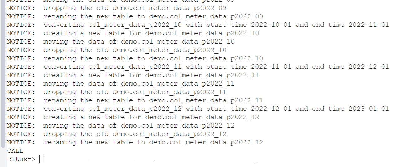
After the function has finished, the table size is now 30GB, down from 117GB. Almost ¼ the size of the ‘heap’ stored data. Pretty impressive for sure. As mentioned above, there are some limitations that exist today with the columnar storage feature but for this use case, or any use case when, after a specified period of time, there will be no further updates to data this is a great solution for reducing storage requirements and increasing query performance in general and for specific analytical aggregate queries as we will see in the testing.

Another useful UDF we have provided, that simplifies partition management is ‘drop_old_time_partitions’. Called like this;

call drop_old_time_partitions(‘meter_data’, now() – interval ‘3 years’);

It would result in any/all partitions older than 3 years being dropped. The nice thing about this is that it doesn’t generate any transaction load on the server. It is simply a metadata operation.

For reference, all the utility functions mentioned in this article are detailed here ;

https://docs.citusdata.com/en/stable/develop/api_udf.html?highlight=shard_count#citus-utility-functions

Ok, back to the testing. We ran all 4 queries on each of the 2 tables on both configurations. Both the heap table ‘meter_data’ and the columnar table ‘col_meter_data’. The results are in the following table;

Query	Storage	Config	Run 1	Run 2	Run 3	Run 4	Run 5	Average (Seconds)
1	Heap 1	1	29.9	30.7	31.3	26.8	51.8	34.1
	Columnar 1	1	3.2	2.6	2.4	2.4	9.1	3.94
	Heap 2	2	7.3	1.2	1.2	1.2	1.2	2.42
	Columnar 2	2	0.9	0.5	0.6	0.6	0.8	0.68
2	Heap 1	1	201	155	156	155	156	164.6
	Columnar 1	1	14	5.5	5.3	5.1	5	6.98
	Heap 2	2	131	23	7.7	6.4	6.9	35
	Columnar 2	2	2.6	0.8	0.6	0.7	0.9	1.12
3	Heap 1	1	76	106	112	132	121	109.4
	Columnar 1	1	34	33	18	18	40	28.6
	Heap 2	2	2.1	1.7	1.7	1.7	1.7	1.78
	Columnar 2	2	2.5	2.2	2.2	1.9	2.2	2.2
4	Heap 1	1	117	108	137	137	121	124
	Columnar 1	1	91	86	90	83	83	86.6
	Heap 2	2	7.7	7.7	8.1	7.8	7.8	7.82
	Columnar 2	2	7.5	7.4	7.3	7.3	7.2	7.34

 

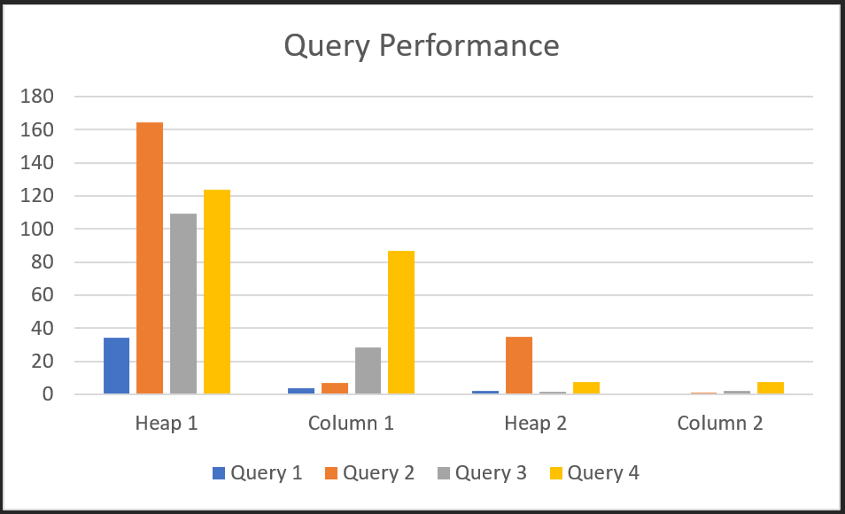
Here is a chart that summarizes the data from the table above, using the average column;

 

Test Summary:

Two things are clear from these tests;

• • Columnar storage outperforms heap storage by a large margin in certain scenarios
  • Distributing such workloads leads to impressive performance gains

Given the enormous scalability on offer with Azure Cosmos DB for PostgreSQL, we believe that it is no longer necessary to send or copy your data to a downstream analytics solution to perform the typical aggregations associated with ‘Analytics’. You have the option of running these aggregates in real time, on a schedule or even via a database trigger. Not only will this solution be capable of scaling to handle truly massive amounts of data, but it can also be considerably less complex and costly than a ‘split’ system handling transactions and analytics in separate databases.

Article Summary:

Ok, there you have it ! A managed open source distributed PostgreSQL service, that scales beyond practically any other relational database and it can handle;

• • Transactions (OLTP)
  • Timeseries
  • IoT
  • Near real-time analytics
  • Columnar storage
  • Geospatial
  • Schema flexibility with JSON datatypes
  • ANSI SQL
  • And even the often touted, less frequently delivered, Hybrid Transactional and Analytical Processing (HTAP)

….and you don’t have to give up on all the features you want from your database like ACID Compliance, Foreign Keys, Joins, Stored Procedures etc.

About Azure Cosmos DB

Azure Cosmos DB is a fully managed and serverless distributed database for modern app development, with SLA-backed speed and availability, automatic and instant scalability, and support for open-source PostgreSQL, MongoDB, and Apache Cassandra. Try Azure Cosmos DB for free here. To stay in the loop on Azure Cosmos DB updates, follow us on Twitter, YouTube, and LinkedIn.

Try Azure Cosmos DB free with Azure AI Advantage

Sign up for the Azure AI Advantage! The Azure AI Advantage offer is for existing Azure AI and GitHub Copilot customers who want to use Azure Cosmos DB as part of their solution stack. With this offer, you get 40,000 free RUs, equivalent of up to $6,000 in savings.