• Part One: Understanding Supply Chains
• Part Two: Enabling SQL Graph
• Part Three: Reaping Graph Rewards ⬅️ You are here.
• Part Four: Visualizing a Graph

Part 3: Reaping Graph Rewards

Clarity

MATCH provides data engineers with a level of clarity that was previously elusive. This clarity is the ultimate value of a graph database, allowing technical information to be communicated precisely and effectively to business stakeholders. By comparing standard join queries to those utilizing MATCH’s declarative join syntax, the advantages become evident.

-- what products are in which stores?

SELECT DISTINCT Product.Name, Store.Name
FROM Plant
JOIN Produces ON Plant.$node_id = Produces.$from_id
JOIN Product ON Produces.$to_id = Product.$node_id
JOIN Delivers_to ON Plant.$node_id = Delivers_to.$from_id
JOIN Warehouse ON Delivers_to.$to_id = Warehouse.$node_id
JOIN Ships_to ON Warehouse.$node_id = Ships_to.$from_id
JOIN Warehouse AS Center ON Ships_to.$to_id = Center.$node_id
JOIN Stocks ON Center.$node_id = Stocks.$from_id
JOIN Store ON Stocks.$to_id = Store.$node_id

-- what products are in which stores?

SELECT DISTINCT Product.Name, Store.Name
FROM Plant, produces, Product, delivers_to, Warehouse, ships_to, Warehouse AS Center, stocks, Store
WHERE MATCH(Product<-(produces)-Plant-(delivers_to)->Warehouse-(ships_to)->Center-(stocks)->Store)

Read more at: SQL Graph JOIN CLAUSE Online Documentation

Consider two identical queries: the first using standard joins, and the second utilizing MATCH. Which one is easier to write? Which one is easier to validate? Which one can be optimized by the engine because it does not explicitly indicate each step of the join? The answer to all those questions is MATCH.

Validation

Validating data and uncovering missing relationships using graphs is straightforward. For instance, a simple question like, “So, Mr. Plant Manager, does this Plant deliver Product 1 to Warehouse 2?” can yield valuable insights. However, be prepared for unexpected feedback, such as, “Actually, we deliver to the Cross Dock down the street, and they handle Product 1’s transfer to Warehouse 2, but only on Tuesdays.” In an instant, your supply chain data becomes more accurate and enriched.

Read more at: Microsoft Whiteboard at the Windows Store

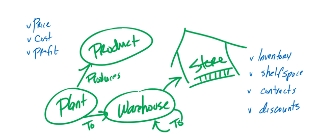
Validating graph data and uncovering missing relationships is made effortless because we communicate using the same language as our business counterparts. Stakeholders can easily analyze the graph and intuitively identify issues and gaps. It’s like drawing on a whiteboard, as a graph essentially consists of circles representing nodes and lines connecting them. From our technical perspective, these circles and lines are SQL tables. However, there’s no need to break the fourth wall with stakeholders; after all, it’s their supply chain we’re discussing.

Discovery

The simplicity of graphs brings another valuable aspect: discovery. In the previous example, we encountered the concept of the Cross Dock for the first time. As we engage in discussions about the relationships between nodes, stakeholders read, validate, and even extend them. For instance, they may provide feedback like, “According to the graph, the Plant produces a certain number of boxes of Product 1. However, in our upgraded systems from last year, we can only measure quantities in Pallets.” Once again, your supply chain data becomes more refined and accurate.

The mere act of examining the graph can inspire further discovery. Stakeholders, in their quest to find answers, start to identify gaps or identify false relationships. The graph’s inherent comprehensibility allows for this organic discovery process to flourish, eliminating the need for constant translation. It is the combination of clarity and validation that fuels the spirit of discovery.

Simplification

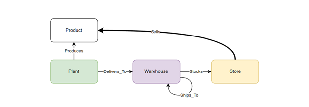
Simplification is the defining characteristic of graphs, and its true power becomes apparent when you eliminate the need to list intricate “systems” within your graph. Consider the relationship “Store-(sells)->Product.” This relationship can elegantly encapsulate complex components such as your purchase order system, third-party vendors in charge of merchandising, and historical store inventory data. All of these elements are consolidated into a concise and meaningful edge labeled “Sells.” While this achievement may require the expertise of your data engineers, it showcases the beauty of graph representation.

Time-based data

Consider the properties you would include in the “sells” edge. Quota? Available Discounts? Quantity Sold? Inventory? Item Price? Now, think about how these values will evolve over time. Handling time-based edges can be challenging. Here are some approaches to consider, keeping in mind that the choice ultimately depends on your business operations. And, if it’s not already apparent, be open to adopting multiple time strategies if necessary.

1. Introduce a date node for nodes: Within your graph, incorporate a date node that represents a specific year, quarter, month, or date—depending on your requirements. Establish a date-oriented relationship from any node to this date node to define the timeframe. However, remember that this solution only addresses dates within nodes. Since edges can only have one “from” and one “to” node, an alternative solution is needed for time-based edges.
2. Incorporate date ranges in the edge: Many databases employ the use of properties like “DateFrom” and (usually nullable) “DateTo” to represent date ranges. Include these properties in your edge structure. This allows you to construct queries with date range logic, similar to what you likely already utilize in your warehouses.
3. Treat your graph as current: Embrace the notion that your graph represents the current state of your business. Since you can have multiple graphs—an approach that is highly recommended—you can create one graph that reflects the present condition of your operations, then another as needed. For example, you might have another graph dedicated to the previous fiscal year. Adopting this perspective simplifies queries and provides a streamlined approach.

CREATE TABLE sells 
(
    Units INT
  , DateFrom DATETIME2
  , DateTo DATETIME2
  , Current BIT
) AS EDGE;

ALTER TABLE sells ADD CONSTRAINT EC_SELLS CONNECTION (Store TO Product)

Supply chain problems

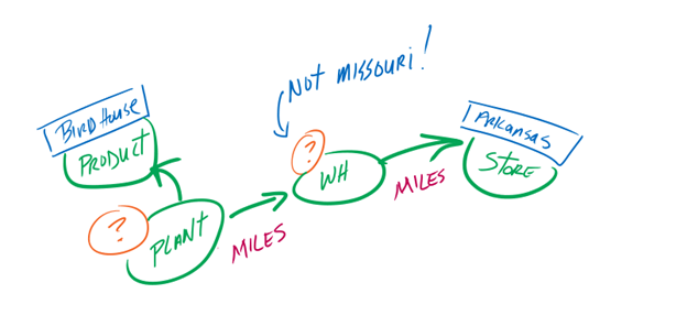
Now that we have our supply chain modeled in a graph, let’s explore a query related to sourcing products for our stores. Specifically, let’s find the shortest paths between a plant and our Arkansas Store. To make it more interesting, we’ll assume there’s an issue with our Missouri Warehouse, so we’ll avoid it.

SELECT 
    Product.Name AS Product
  , Store.Name AS Store
  , CONCAT(Plant.Name, '>', Warehouse.Name, '>', Store.Name) AS ShipPath
  , FORMAT(delivers_to.Miles + stocks.Miles, 'N0') AS Miles

FROM Plant, produces, Product, delivers_to, Warehouse, stocks, Store

WHERE MATCH(Product<-(produces)-Plant-(delivers_to)->Warehouse-(stocks)->Store)
  AND Warehouse.Name <> 'MO'
  AND Product.Name = 'Bird House'
  AND Store.Name = 'AR'

ORDER BY delivers_to.Miles + stocks.Miles

This query involves joining tables such as Plant, produces, Product, delivers_to, Warehouse, stocks, and Store. By using the MATCH statement to describe the relationships, SQL’s graph engine takes care of the rest. There’s no need for advanced graph algorithms—this query beautifully showcases how MATCH declares relationships between tables. Just imagine how easy it would be to validate this query with stakeholders. You can even draw it on a whiteboard to demonstrate the simplicity of the process.

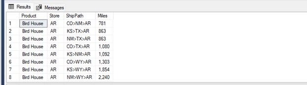
Under analysis, our results indicate that the best plant for manufacturing Bird Houses for the Arkansas Store is located in Colorado. Furthermore, if we route through Texas, we find that Kansas offers a modest improvement. This secondary insight becomes valuable in the event of capacity issues at the Colorado Plant or other considerations. It’s not magic—it’s simply the power of simplicity. Our data and queries become easier to communicate and understand.

Just the beginning

It’s worth pointing out that none of this this demonstration showcases the exotic features of SQL Graph—such as graph algorithms enabling recursive SHORTEST_PATH lookups. Instead, our focus lies on the inherent benefits of the graph paradigm: aligning data directly with the workings of the business and enabling stakeholders to communicate using familiar terminology. All of this is achieved without compromising the robustness and familiarity of SQL Server, where your data already resides. You can enjoy the manageability, security, integration, and extensive ecosystem of tools that SQL Server offers. It truly combines the best of both worlds.

Conclusion

In Part 3, we explored the clarity, validation, discovery, and simplification that come with working with graph data in SQL Graph. We discovered that the MATCH keyword provides data engineers with a level of clarity that was previously challenging to achieve. By utilizing the declarative join syntax of MATCH, we can easily write, validate, and optimize queries, enabling effective communication with business stakeholders.

Validation becomes seamless as we use graphs to uncover missing relationships and validate data. Stakeholders can intuitively analyze the graph and identify issues and gaps, eliminating the need for constant translation. The inherent simplicity of graphs fosters discovery, as stakeholders can explore and extend relationships to gain deeper insights into the supply chain. Simplification is another hallmark of graphs, allowing us to consolidate complex systems into concise and meaningful edges.

Looking ahead to Part 4, we will explore the power of graph visualization. We will discover how graph visualization tools, such as the force-directed graph visual in PowerBI, enable interactive and shareable representations of our graph data. Stay tuned to unlock the full potential of graph visualization in gaining a holistic understanding of your supply chain and making informed decisions.