
Now that you’ve had a chance to read the Intro to Indirect Time-of-Flight (ToF) post, let’s dig a little deeper into the mechanics behind the Microsoft implementation of time-of-flight depth sensing, as well as a couple functional advantages it presents.
How does “Indirect” ToF work?
To recap, “time-of-flight” refers to emitting light at an object and measuring how long it takes to bounce back and return, then converting the time measurement into distance using the speed of light, giving us the object’s shape and position in its surroundings.
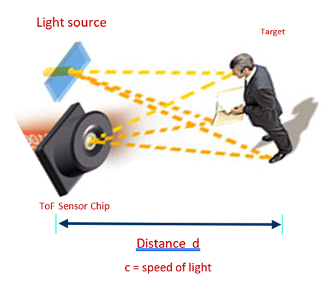
Figure 1. Generalized operation of time-of-flight sensing.
In practice, we don’t use the actual round-trip time – to get millimeter precision, we would need picosecond stopwatch circuits for every pixel! Instead, we take the “indirect” approach, where we emit light with a periodic or “modulated” pattern, then calculate the shift in the return measurement.
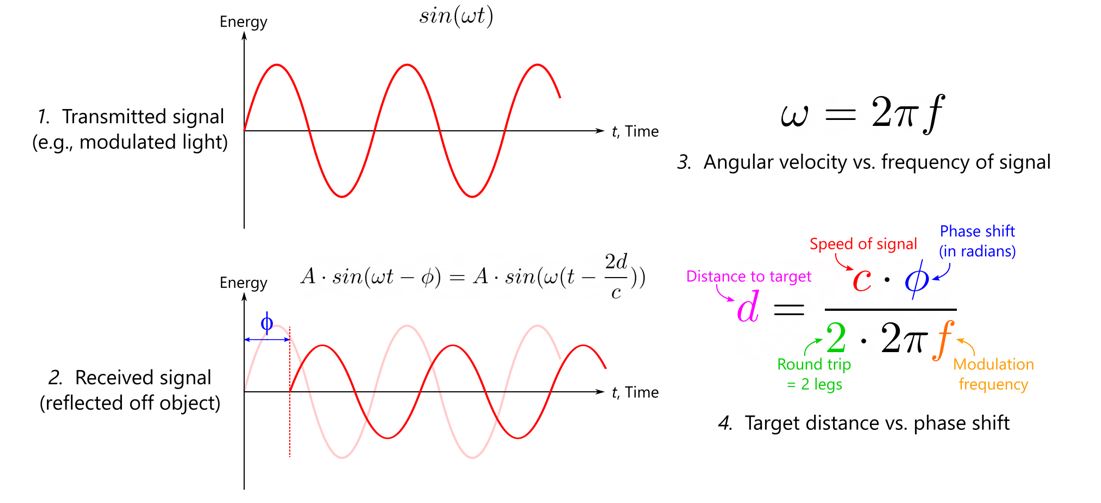
Figure 2. Plots of modulated signal energy as time elapses, both transmitted and received, and the mathematical relationship between phase shift and distance.
How do we measure this phase shift? At the silicon level, each pixel in the Microsoft ToF sensor is comprised of two detectors, or “wells”, that receive photons and turn them into electric charge. Each well can be opened or closed by the sensor control circuit. If we keep each well open for half of a modulation period – side A in sync with the emitter, and side B exactly out of sync – then the returning photons will be split between the two detectors, but at least one well is always ready to catch them. Based on the proportion of photons that accumulate in detector A vs. detector B, we can calculate the shift of the returned signal. (We wait for the modulation period to repeat a few times to accumulate charge – this is referred to as “integration time”, much like shutter speed on a color camera.)
Figure 3a. Animation showing the synchronized emitter-sensor operation. Modulated light leaves the emitter on the far right, strikes the target on the left, and returns to a certain pixel in the sensor on the middle-right. Detector A (in green) is open while the emitter is active, and Detector B (in cyan) is open during the inactive part of the cycle. Because of the phase shift, returning photons will not necessarily arrive in sync.
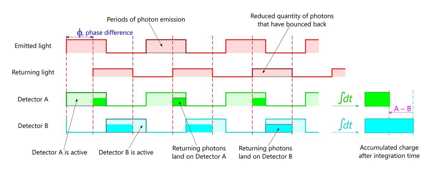
Figure 3b. 2D plots of light energy over time in the same scenario. The difference in accumulated charge between the two detectors will be the “output” of this pixel.
Is one measurement enough?
However, we can’t stop here. If a second object appears in the scene, at a distance that gives it the same phase shift but the opposite direction, what happens? The split of accumulated charge in the pixel is just like it was before, but we have no way to know that detector A was charged at the end of the return instead of the beginning. This means that our measurement is ambiguous.
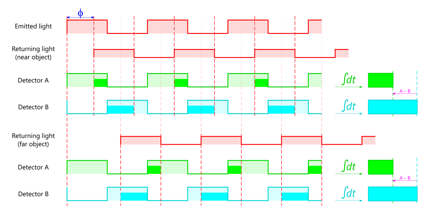 Figure 4. The same scenario as above, but contrasted with a hypothetical second target that’s about one-third of a modulation period farther away. Our (A – B) output has not changed…
There are a few ways to remove the ambiguity. The most common method is to repeat the measurements immediately, but push the sensor out of phase, filling out the picture of the returned wave. In this example, we modulate the sensor 90 degrees out of phase with respect to the light source, changing the open-close pattern of the charge accumulators in the pixel:
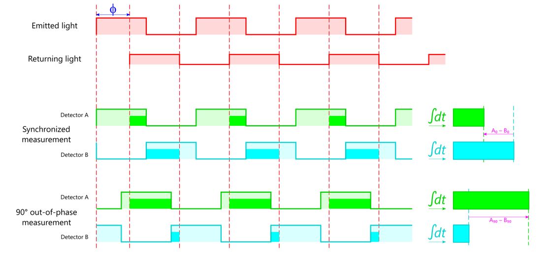
Figure 5. Another pair of measurements in the original scenario adds information that can be used to disambiguate.
Seeing how the returned light “projects” itself onto the synchronized and 90-degree wells, we can use complex numbers to reconstruct the original phase shift, discarding the false second solution. This complex sum gives us both the phase shift (angle from the real axis) we were originally after and the brightness of the returned light (as the magnitude of the complex number). From this brightness calculation, we can extract object reflectivity, or monochrome images of the scene in infrared!
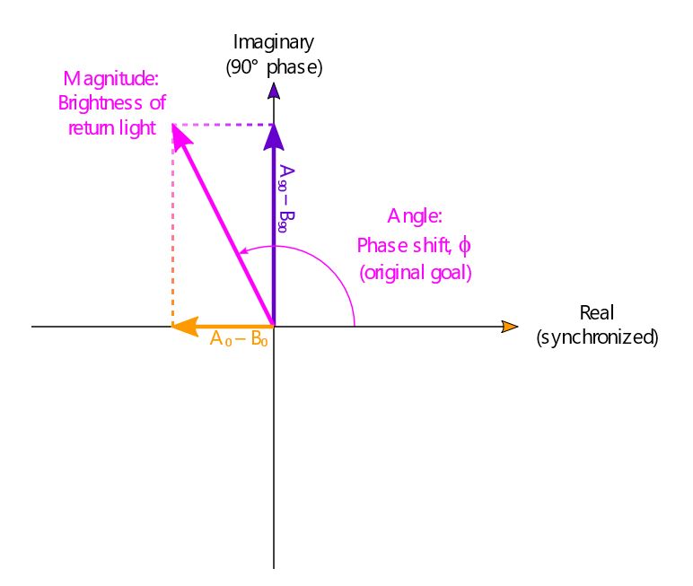
Figure 6. Combining the two difference measurements from the pixel.
What about other sources of light?
Now consider a case where the modulated light from our camera is not the only light present in the scene. It’s common for other sources, such as the sun, to provide “ambient” light strong enough to show up in our measurements. This has a diluting effect, dropping extra photons onto our detectors whenever they are open.
Since this extra light is generally unmodulated, it will impact both detectors about equally. However, our phase shift measurements depend only on the difference between the two, which means that we can tolerate a lot of ambient light without introducing a systematic bias! Not only that, we don’t have to dynamically tailor our shutter speed to the environment, unless we observe light levels so high that pixels are “saturating”, or completely filling the charge wells during an exposure. These benefits of differential measurement turn a lot of potentially challenging scenarios into plug-and-play simplicity.
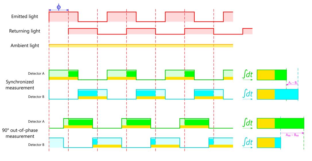
Figure 7. The ambient light energy contributes about the same offset to each detector measurement, leaving the difference unaffected.
Now, I hate to attenuate the sunny overview we’ve had so far, but it’s important to note that the indirect time-of-flight system is not without its sources of error. Ambient light may not cause interference by matching up with modulation, but it still adds its own variation, or “noise”, to the measurements. There is also noise in the system itself – pixels may respond more strongly or weakly to the same amount of light; the light source can experience time or intensity fluctuations. If ambient light begins to overfill the pixels, it compresses the space that the two wells need to differentiate themselves from each other, which intensifies the effect of any noise contributions. We can’t completely avoid this, but to reduce it, we select a wavelength for our emitter from an atmospheric absorption band, and add a sensor bandpass filter to help screen photons we didn’t produce ourselves.
In conclusion, differential response of modulated light as an indirect time-of-flight measurement brings a lot to the table, even in this basic form: robust accuracy even in the presence of extra light, performance without much prior knowledge of the environment, additional measurement streams such as reflectivity and monochrome IR imaging. In future posts, we’ll cover even more benefits of our ToF sensor and the improvements that we made on the basic indirect ToF mechanism.
0 comments