Modeling quantum architecture with Azure Quantum Resource Estimator

Ivan Basov

Introduction

There are numerous architectural decisions to consider when building quantum computers, which have the potential to address real-world computational challenges like quantum chemistry and quantum cryptography. Researchers worldwide are engaged in developing various aspects of quantum computer architecture. Microsoft Azure Quantum Resource Estimator plays a pivotal role in assessing how different combinations of design choices might impact the performance of upcoming quantum computers.

Azure Quantum Resource Estimator was designed to assist researchers in estimating computational time and the requisite number of qubits based on diverse assumptions regarding hardware quality and error correction strategies. We have used a more powerful version of the Resource Estimator for many years as an internal tool for analyzing architectural decisions in our own quantum program. We have incorporated new options to offer similar capabilities to the Azure Quantum users.

Continuing our commitment to enhancing the tool’s capabilities, we have recently introduced several new features. These updates include the ability to customize error budget distributions and implement custom distillation units.

In this article, we provide an overview of fundamental concepts related to the architecture of quantum computers, exploring their influence on the necessary resources and the capabilities offered by Microsoft Azure Quantum Resource Estimator to model these intricate structures.

One can represent quantum computing stack as follows:

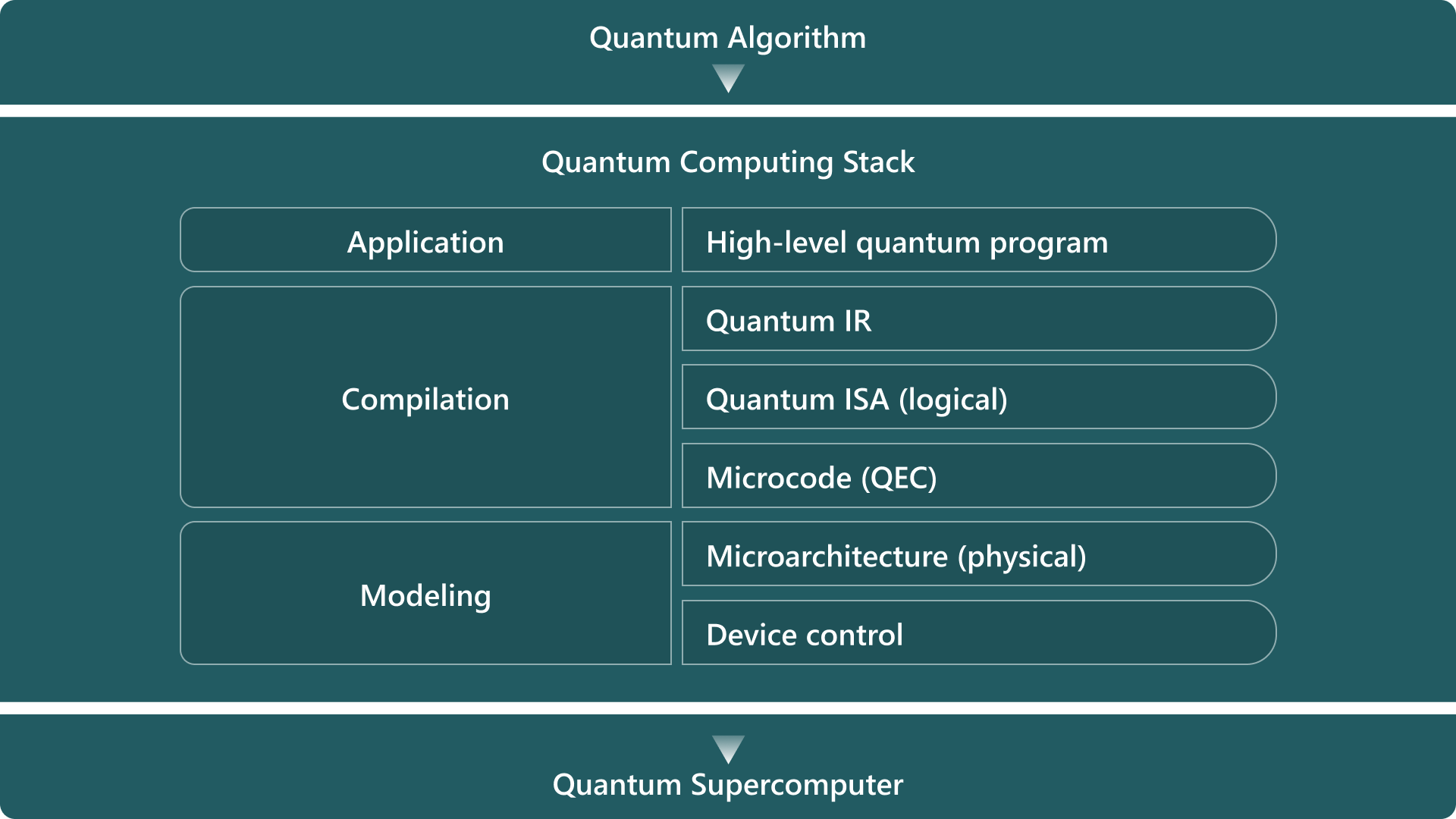
Scientists all around the world are collaborating on refining individual stack components and integrating them cohesively. The multitude of decisions made at each stack layer, coupled with diverse quantum algorithms, results in a vast array of possible combinations that warrant evaluation and comparison. Microsoft Azure Quantum Resource Estimator helps to assess and compare those combinations efficiently. You can submit your quantum program (such as in Q# or Qiskit) or Quantum Intermediate Representation (QIR) while specifying particular characteristics of a proposed quantum computing stack:

• Microarchitecture of magic state distillation and physical qubit parameters
• Quantum error correction
• Error budget allowed for the program

And the Resource Estimator will calculate rQOPS of the architecture and, qubits and time required for the application given this combination.

Physical qubit parameters

In the current landscape of 2023, a significant challenge lies in the pursuit of rapidly responsive, stable, and scalable physical qubits to enable impactful applications in chemistry and materials science (read more at Communications of the ACM, 2023). Researchers are exploring a range of design possibilities, including instruction sets as well as diverse anticipated levels of speed and fidelity for these qubits. 

In the process of resource estimation, a higher degree of specificity becomes necessary, encompassing various times for distinct actions involving qubits. Our recent updates here involve:

• Providing separate `process` and `readout` error rates for qubit measurements;
• Adding an idling error rate to the model;
• Separating `Clifford` and `readout` error rates in magic state distillation formulas.

Azure Quantum Resource Estimator supports:

• predefined qubit types with characteristics expected or targeted,
• and custom qubit types where users could provide specific times and error rates.

Here is an example of specifying a custom qubit type:

from azure.quantum import Workspace
from azure.quantum.target.microsoft import MicrosoftEstimator
from azure.quantum.target.microsoft.target import MeasurementErrorRate

#Enter your Azure Quantum workspace details here
workspace = Workspace(
    resource_id="",
    location=""
)

estimator = MicrosoftEstimator(workspace)
params = estimator.make_params()
params.qubit_params.name = "qubit_maj_ns_e6"
params.qubit_params.instruction_set = "Majorana"
params.qubit_params.one_qubit_measurement_time ="150 ns"
params.qubit_params.two_qubit_joint_measurement_time = "200 ns"
params.qubit_params.t_gate_time = "100 ns"
params.qubit_params.one_qubit_measurement_error_rate = MeasurementErrorRate(process=1e-6, readout=2e-6)
params.qubit_params.two_qubit_joint_measurement_error_rate = 1e-6

# test quantum program
from qiskit import QuantumCircuit
circ = QuantumCircuit(3)
circ.crx(0.2, 0, 1)
circ.ccx(0, 1, 2)

job = estimator.submit(circ)
job.wait_until_completed()
result = job.get_results()
print(result)

We use a simple Qiskit circuit for this blog post for short. To learn how to run resource estimator for Q# algorithms, go to the Create the quantum algorithm section at the resource estimator documentation.

You can learn more about this at the Physical qubit parameters section of documentation. 

Quantum error correction

Error correction in classical computing involves creating duplicates or checksums of data and periodically verifying these duplicates. In quantum computing, error correction is more complex due to the impossibility of copying information (see No-cloning theorem).

However, the basic principles are similar to classical error correction: achieving greater accuracy in computations requires extra resources (additional qubits and time). Analogous to classical computing, the extent of extra information can be quantified using a code distance (see Hamming distance). Opting for a higher code distance necessitates more resources but leads to enhanced computation fidelity.

We use the following exponential model for error rate suppression:

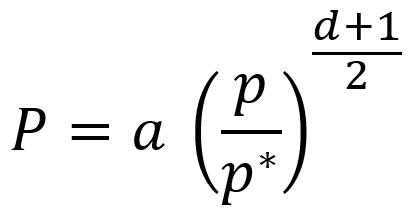
Here, p – is the physical qubit error rate (computed from various physical error rates above), P – is the (output) logical error rate provided by an error correction scheme, d – is the code distance, and a and p – are coefficients specific for the scheme, called crossing prefactor and error correction threshold correspondingly. As you can see, if p < p*, then P increases when d increases.

As mentioned above, resources involved would also grow with increasing of d. Here are examples for the Floquet scheme (arxiv.org:2202.11829):

logicalCycleTime=3 * oneQubitMeasurementTime * d,
physcialQubitsPerLogicalQubit=4 * d^2 + 8 * (d -1).

Microsoft Azure Quantum Resource Estimator supports two predefined schemes of error correction: surface and Floquet, as well as custom error correction schemes.

The surface scheme is based on the premise that physical qubits form a lattice on a surface. In this arrangement, we have two types of qubits: data qubits, which play a role in primary algorithm computations, and measurement qubits, which serve as supplementary components. These qubits are organized in a checkerboard pattern, where each data qubit is surrounded by four measurement qubits, and vice versa. Boundary qubits are conceptually linked to qubits on the opposite side, creating a toroidal structure. Stabilization measurements are performed on corresponding qubits along different axes with a specific geometric pattern. This scheme exhibits versatility, as it can be applied to both gate-based qubits and Majorana qubits.

Conversely, the Floquet scheme places more stringent demands on the geometric arrangement of qubits but offers significant advantages in terms of time and space efficiency (as detailed in arxiv.org: 2202.11829). Qubits must be arranged in a grid with three neighbors each, and it should be possible to color the plaquettes with just three colors. Honeycomb is an example of such structure. Subsequently, stabilization measurements are executed periodically with a period of three, involving joint measurements between one qubit and one of its three neighbors at a time. This geometric structure aligns well with Majorana qubits and can bring substantial benefits when applied to them.

If using Microsoft Quantum Development Kit, one can submit the following job with different error correction schemes:

from azure.quantum import Workspace
from azure.quantum.target.microsoft import MicrosoftEstimator, ErrorBudgetPartition

# Enter your Azure Quantum workspace details here
workspace = Workspace(
    resource_id="",
    location=""
)

estimator = MicrosoftEstimator(workspace)
params = estimator.make_params()
params.qec_scheme.error_correction_threshold = 0.01
params.qec_scheme.crossing_prefactor = 0.07
params.qec_scheme.logical_cycle_time = "3 * oneQubitMeasurementTime * codeDistance"
params.qec_scheme.physical_qubits_per_logical_qubit = "4 * codeDistance * codeDistance + 8 * (codeDistance - 1)"

# there are two predefined schemes: floquet_code and surface_code
# the floquet_code can be applied for models with Majorana instruction set
# the surface code can be applied to both: Majorana and gate-based instruction sets.
# you can just specify the name of a predefined scheme

#params.name = "surface_code"

# test quantum program
from qiskit import QuantumCircuit
circ = QuantumCircuit(3)
circ.crx(0.2, 0, 1)
circ.ccx(0, 1, 2)

job = estimator.submit(circ)
job.wait_until_completed()
result = job.get_results()
print(result)

See more at the Quantum error correction schemes section of the Resource Estimator documentation.

Magic state distillation

To harness the benefits of quantum computing over classical counterparts, it is essential to devise quantum gates that cannot be effectively simulated on traditional non-quantum hardware. These operations can be envisioned as rotations of the Bloch sphere, executed at arbitrary angles. In this context, classical non-quantum hardware is proficient at executing rotations limited to angles of 90 degrees. This particular set of operations can be encapsulated by the concept of Clifford gates.

By combining a set of Clifford gates with additional non-Clifford gates, it is possible to create a universal set of quantum gates. This means that any quantum gate can be efficiently approximated to the desired precision using a predefined sequence of operations from this set. This approximation process is commonly referred to as rotation synthesis.

Various quantum computer architectures might incorporate distinct non-Clifford gates within the rotation synthesis. These particular gates are often termed “magic gates,” and their associated states are labeled as “magic states.” A notable challenge in quantum computing stems from its inherent inability to duplicate data. Consequently, generating these magic states once and employing them indefinitely is unfeasible. Instead, each usage demands the creation of fresh instances of these magic states. This intricate procedure of generating magic states with a specified level of precision is known as magic state distillation.

One of popular choices for the magic state is the T-gate defined as follows: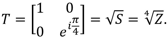

In Azure Quantum Resource Estimator, we assume that the T-state is used as the magic state.

Algorithms designed for T-state distillation play a crucial role in enhancing qubit accuracy. These algorithms utilize multiple input qubits with low accuracy to generate an output qubit with higher accuracy. This process can encompass multiple rounds of distillation, progressively refining qubit quality until the desired standard is attained. Each round employs a specific algorithm known as a distillation unit.

For each distillation unit, one should specify how it improves the qubit quality and what resources it will consume for the runtime: qubits involved, and time spent. Those characteristics depend on the code distance used for the distillation, physical quality of qubits and accuracy provided originally or by the previous round of distillation.

It’s important to note that distinct sequences of distillations can yield greater efficiency for different qubit qualities (output error rates). In other words, depending on the initial error rate of an input qubit, specific sequences of distillation may be more adept at achieving the required error rate while utilizing fewer resources.

Here are examples of distillation units described in Assessing requirements to scale to practical quantum advantage:

When we are estimating the performance of a particular quantum algorithm on a specific quantum computer (which has a certain qubit quality and operation speed), we might need different target output error rates. Considering two distillation units (15-to-1 space-efficiency and 15-to-1 RM preparation) and various code distances for each round, there could potentially be thousands of combinations to evaluate.

Various research groups are actively working on developing distillation algorithms, and their approaches might differ from the ones described earlier. For instance, some algorithms could generate multiple output T-states, potentially reducing costs by sharing resources or enabling parallelization. With dozens of distillation algorithms in consideration, an intriguing opportunity arises to compare them against each other, encompassing diverse physical qubit attributes and algorithm variations. This comparative analysis could provide valuable insights into their relative effectiveness.

Microsoft Quantum invites researchers to assess the resources needed for their unique distillation approaches. Presently, we offer support for two established distillation units named `15-1 RM` and `15-1 space-efficient`, in addition to the flexibility to define custom distillation unit specifications.

Here is an example of calling the Resource Estimator with custom distillation unit specifications:

from azure.quantum import Workspace
from azure.quantum.target.microsoft import MicrosoftEstimator
from azure.quantum.target.microsoft.target import DistillationUnitSpecification, ProtocolSpecificDistillationUnitSpecification

# Enter your Azure Quantum workspace details here
workspace = Workspace(
    resource_id="",
    location=""
)

estimator = MicrosoftEstimator(workspace)
params = estimator.make_params()
specification1 = DistillationUnitSpecification()
specification1.display_name = "28-2"
specification1.num_input_ts = 2
specification1.num_output_ts = 28
specification1.output_error_rate_formula = "35.0 * inputErrorRate ^ 3 + 7.1 * cliffordErrorRate"
specification1.failure_probability_formula = "15.0 * inputErrorRate + 356.0 * cliffordErrorRate"

physical_qubit_specification = ProtocolSpecificDistillationUnitSpecification()
physical_qubit_specification.num_unit_qubits = 12
physical_qubit_specification.duration_in_qubit_cycle_time = 65

specification1.physical_qubit_specification = physical_qubit_specification

logical_qubit_specification = ProtocolSpecificDistillationUnitSpecification()
logical_qubit_specification.num_unit_qubits = 20
logical_qubit_specification.duration_in_qubit_cycle_time = 37
specification1.logical_qubit_specification = physical_qubit_specification

specification2 = DistillationUnitSpecification()
specification2.name = "15-1 RM"

specification3 = DistillationUnitSpecification()
specification3.name = "15-1 space-efficient"

params.distillation_unit_specifications =[specification1, specification2, specification3]

# test quantum program
from qiskit import QuantumCircuit
circ = QuantumCircuit(3)
circ.crx(0.2, 0, 1)
circ.ccx(0, 1, 2)

job = estimator.submit(circ)
job.wait_until_completed()
result = job.get_results()
print(result)

For further information, please refer to the Distillation Units section in the Resource Estimator documentation.

Error budget

Quantum algorithms inherently embrace a probabilistic aspect, and the execution process is susceptible to errors. Typically, an algorithm can be run multiple times to reveal its probabilistic behavior and mitigate errors. When sending an algorithm for quantum computer execution, it’s crucial to determine how many runs are required to achieve a desired confidence level. Consequently, a probability of error in the final computations is defined, termed the error budget. Seeking a higher probability of success can involve employing the error correction methods elucidated earlier. However, it is important to note that this pursuit of higher success probability comes at an elevated cost, involving more qubits and a longer runtime.

We could categorize errors into three categories by occurrence:

• During distilling magic states
• During performing rotations
• While executing the algorithm

As an initial approximation, we might distribute the error budget evenly among these three sources. Yet, certain algorithms could demand varying amounts of rotations or magic states. Hence, there could be a preference to readjust the error budget to align with the intricacies of the algorithm in question.

If using Microsoft Quantum Development Kit, one can submit the following job with different error budget options:

from azure.quantum import Workspace
from azure.quantum.target.microsoft import MicrosoftEstimator, ErrorBudgetPartition

# Enter your Azure Quantum workspace details here
workspace = Workspace(
    resource_id="",
    location=""
)  

estimator = MicrosoftEstimator(workspace)
params = estimator.make_params()

# make an estimate with specific error budget
# for each of the three error sources:
params.error_budget = ErrorBudgetPartition(logical=0.001, t_states=0.002, rotations=0.003)

# for uniformly distributed error budgets,
# # you can specify just the total as single number:
# params.error_budget = 0.001

# test quantum program
from qiskit import QuantumCircuit
circ = QuantumCircuit(3)
circ.crx(0.2, 0, 1)
circ.ccx(0, 1, 2)

job = estimator.submit(circ)
job.wait_until_comps()
print(result)leted()
result = job.get_result

Read more about error budgets in the documentation.

Conclusion

The Azure Quantum team is dedicated to ongoing enhancements of the Resource Estimator. This valuable tool serves both our internal teams and external researchers in the endeavor to design quantum computers. Expanding the scope of modeling capabilities remains a key priority for us. We eagerly welcome your feedback on the specific custom options you require for estimating your quantum computer resources. Your insights will greatly contribute to refining our tool and making it even more effective for the quantum community.

Learn more about Resource Estimation

There are many ways to learn more:

• Visit our technical documentation for more information on Resource Estimation, including detailed steps to get you started.
• Login to the Azure Portal, visit your Azure Quantum workspace, and try an advanced sample on topics such as factoring and quantum chemistry.
• Dive deeper into our research on Resource Estimation at arXiv.org.

Ivan Basov Principal Quantum Software Engineer, Microsoft Quantum

Follow