

Introduction
During one of our recent projects, we were working with an advertising customer. They were aiming for 1:1 ad personalization, where each content piece is tailored to each unique customer, but that’s done in a repeatable and measurable way.
Our defined experiments aimed to prove that we can create AI-generated ads that contain real images of products, without editing the supplied image of the product so that it is properly represented.
The following hypothesis is considered a crucial prerequisite in order to be able to reach their goal around effectively scaling image personalization, while maintaining the integrity of the item being advertised.
“Given an image of a product and a text description of its surroundings, we can generate a high-fidelity image with visual elements representing the described environment that includes an unmodified version of the supplied product’s image”
The most promising technology that can accomplish this AI-generated background is ‘inpainting’, a feature of multi-modal text-to-image models. With inpainting, the inputs are:
- An image of the product
- A mask representing the area of the background to be generated
- A textual prompt describing the background to be generated.
The output is an image where the masked area has been generated as a background to the product, according to the textual prompt. The product content may have been slightly modified to fit into the background, especially if the masked areas are close to the product content.
Since the output of inpainting cannot guarantee that the product was not modified, we needed a way to measure if the generated images altered the product.
Experiments
Three measurements techniques were used in determining the delta between the base product image and the generated ad image:
Mean Squared Error (MSE)
MSE measures the average squared difference between the estimated values (predicted values) and the actual values (ground truth). We calculate squared differences pixel by pixel. But this works well only if we want to generate an image with the best pixel colors that conform with the ground truth image.
import numpy as np

product_image_pixels = [[1, 2, 3, 4],[5, 6, 7, 8]]
generated_image_pixels = [[1, 1, 3, 5],[5, 6, 7, 9]]

# Mean Squared Error
mse = np.square(np.subtract(product_image_pixels, generated_image_pixels)).mean()
Peak Signal to Noise Ratio (PSNR)
To use this estimator, we must transform all values of pixel representation to bit form. If we have 8-bit pixels, then the values of the pixel channels must be from 0 to 255. The red, green, blue, or RGB, color model fits best for the PSNR. PSNR shows a ratio between the maximum possible power of a signal and the power of corrupting noise that affects the fidelity of its representation.
import numpy as np

product_image_pixels = [[1, 2, 3, 4],[5, 6, 7, 8]]
generated_image_pixels = [[1, 1, 3, 5],[5, 6, 7, 9]]

mse = np.square(np.subtract(product_image_pixels, generated_image_pixels)).mean()

# Peak Signal to Noise Ratio
psnr = 100 if mse == 0 else 20 * log10(255.0 / sqrt(mse))
Cosine Similarity
Cosine similarity can be used to measure the likeness between different images or shapes. Vector embeddings for images are typically generated using Convolutional Neural Networks (CNN) or other deep learning techniques to capture the visual patterns in the images.
We only use the ’feature learning’ part of the CNN flow for the purpose of comparing the vectors representing the features.
import numpy as np
from tensorflow.keras.applications.vgg16 import VGG16
from keras.models import Model
from keras.preprocessing import image
from keras.applications.imagenet_utils import preprocess_input
from scipy import spatial

def get_feature_vector(img_path):
    # Name of last layer for feature extraction
    feature_extraction_layer = 'fc2'
    model = VGG16(weights='imagenet', include_top=True)
    model_feature_vect = Model(inputs=model.input, outputs=model.get_layer(feature_extraction_layer).output)
    img = image.load_img(img_path, target_size=self.img_size_model)
    img_arr = np.array(img)
    img_arr = np.expand_dims(img_arr, axis=0)
    processed_img = preprocess_input(img_arr)
    feature_vect = model_feature_vect.predict(processed_img)
    return feature_vect

# Compute feature vector extracted
fea_vec_img1 = get_feature_vector(‘product.png’)
fea_vec_img2 = get_feature_vector(‘generated-image.png’)

# Flatten the array from 2d to 1d for cosine processing
fea_vec_img1 = fea_vec_img1.flatten()
fea_vec_img2 = fea_vec_img2.flatten()

# Cosine Similarity
cos_sim = 1-spatial.distance.cosine(fea_vec_img1, fea_vec_img2)
Template Matching
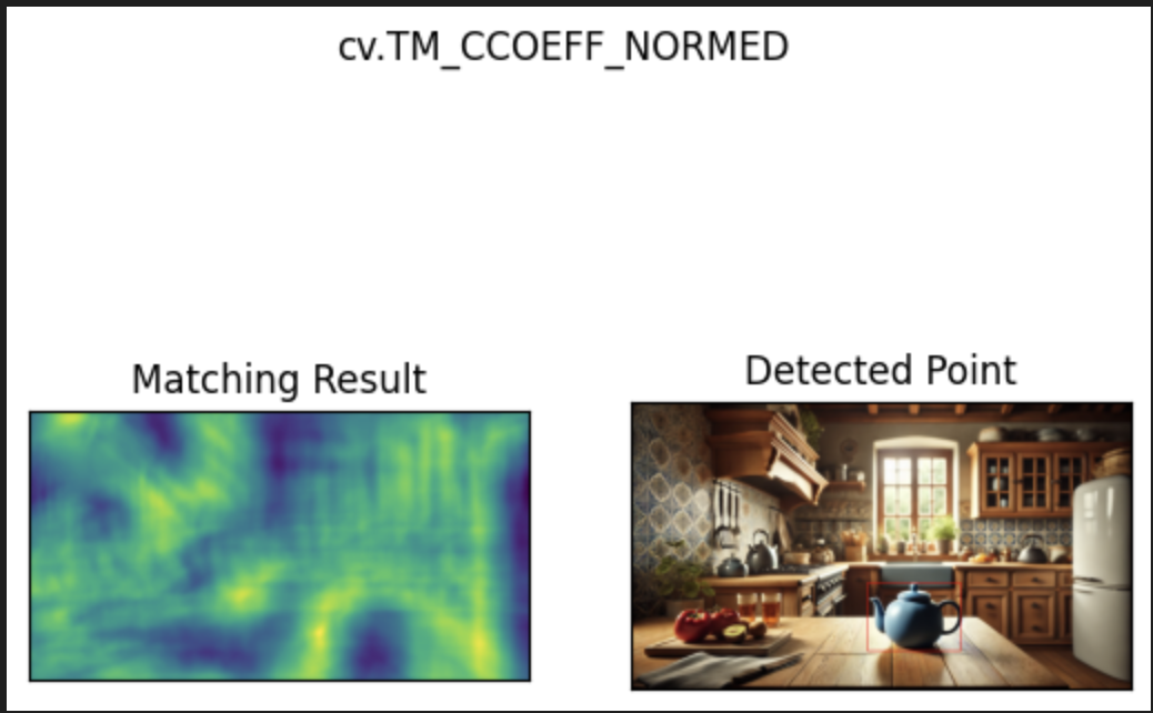
There were also experiments run on detecting where the product exists within the generated image, to compare same-sized images containing the product. This was done using template matching, which is a method used to locate a smaller image (the ‘template’) within a larger image. It works by sliding the template image across the larger image and calculating a similarity score at each position to find a match.
import cv2 as cv

template_img = cv.imread('product.png', cv.IMREAD_UNCHANGED)
generated_img = cv.imread('generated-image.png', cv.IMREAD_UNCHANGED)

# Template Match - Find the location of the product within the generated image
res = cv.matchTemplate(generated_img, template_img, cv.TM_CCOEFF)
_, max_loc = cv.minMaxLoc(res)
top_left = max_loc
h, w = template_img.shape[:2]
bottom_right = (top_left[0] + w, top_left[1] + h)

# Draw a rectangle around the matched region.
cv.rectangle(generated_img, top_left, bottom_right, (255, 0, 0), 5)
Results
Comparators
To test the capabilities of each image comparator technique, a series of benchmark images were used. These are images where the delta between the images is known, such that we can accurately compare expected vs. actual results. The images include tests such as various levels of image fill, transparency fill, content rotation, translation, coloring, and image scaling.
Mean Squared Error
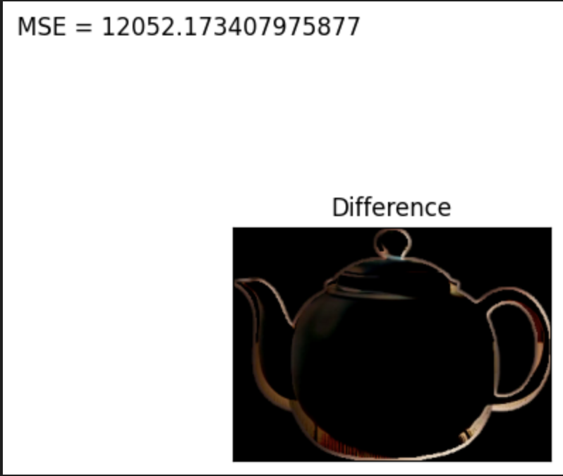
MSE performed well in accurately detecting changes in exact pixel differences, which is to be expected. It considers all pixel RGBA values when evaluating the difference between the images. This means that it performed well in detecting product color and disproportionate scale differences, assuming the product is in the same location in each image.
MSE isn’t useful when the product was translated unless a template matcher is used. This is expected, as it is simply comparing each pixel value of the image. If the product was rotated or proportionately scaled, again MSE will simply find the differences between the pixel values, even if those differences are acceptable.
Peak Signal-to-Noise Ratio
PSNR performed well in detecting changes of pixel differences like MSE, albeit due to the logarithmic nature of the measurements the results can be more difficult to discern. For example, comparing a fully white image against a half white half transparent image one might expect a value of 47 since the range of PSNR is between -6.02 and 100. However, it is -3.01 due to that log part of the calculation. The advantage though of a logarithmic result is that it is easy to tell how many orders of magnitude different the images are. For example if MSE was 10, the result of PSNR is 38.13. If MSE is 100, the result is 28.13 and so on. It performs well in detecting product color and scale differences, assuming the product is in the same location in each image.
Like MSE, PSNR wasn’t useful when the product was translated, unless a template matcher is used. It also can’t discern a product rotation or proportionate scale and will simply report the raw pixel differences like MSE.
Cosine Similarity
Cosine similarity performed well in detecting changes in the edges and curves that define the product. This means that it has less need for a template matcher. So, if the image was translated or proportionately scaled, it will accurately determine if there were changes made to the product itself rather than the whole image.
Like MSE and PSNR though, it isn’t useful when the product is rotated, unless detecting such rotation differences is a desired result as a detected discrepancy against the baseline product image. With a disproportionate scaling comparison, it determines the images to be similar, which is not desired for our use case. This is expected due to how feature matching works, but not particularly useful in detecting when a change was made to a product. It also won’t detect pixel color changes as well as MSE or PSNR due to it only comparing features.
Template Matching
We used OpenCV to find a template in a target image. The template can be located if it is the same size or smaller than the target image and has the same resolution. If the target image and the template have different resolutions, then there is no guarantee the template can be found without some resizing techniques. OpenCV does not keep track of resolution so implementing this functionality would require additional knowledge about the image resolutions. We recommend keeping the resolution the same between the template and the target image. The resolution of the target image will be dictated by the particular GenAI model used so several resolutions of the same template image may be necessary to match the output resolution of the GenAI models.
Experiment Screenshots
Comparator
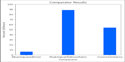
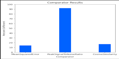
Here are a few of the results of comparator color, translation, rotation, and scale delta experiments:
Color

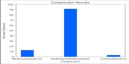
Translation
![]()
![]()
Rotation

Scale

Template Matching
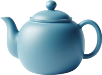
Template image and AI generated image
Template match detected the bounding box at which the template image was found within the AI generated image
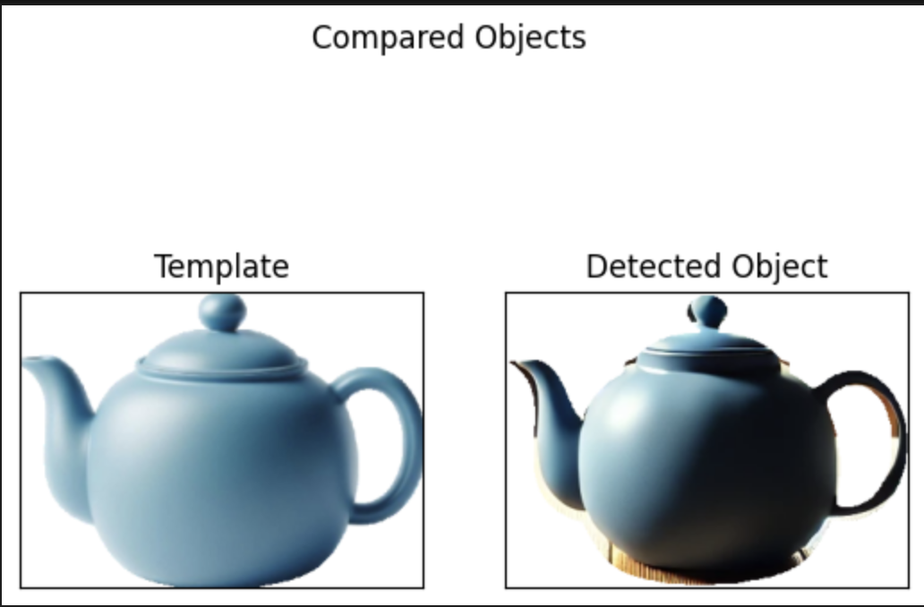
Side-by-side comparison of original product image against the detected product in the generated image
Visualization of the differences between them
Conclusion
With the combination of template matching, MSE, PSNR, and Cosine Similarity, we can achieve a strong system of image comparison to determine whether the product has been edited in the AI-generated image output.
A combination of MSE (or PSNR) and Cosine Similarity comparators can give us meaningful metrics to determine undesired changes between the baseline product image and the generated image. The strength of combining multiple image comparators is that we can leverage the benefits of each, and they complement each other’s shortcomings. With MSE and PSNR, the key benefit is in determining color differences and disproportionate scaling. With Cosine Similarity, the key benefit is determining differences in the edges and curves that define the product, regardless of its location or proportionate scale in the generated image.
Template matching serves to provide a baseline of which to compare the images. By finding where the product is in the generated image, we can scope the comparison of only the relevant pixels. This helps when running MSE and PSNR due to the nature of how those comparison techniques are performed and gives us a more meaningful result from those comparators.
Further Considerations
Further considerations include handling scaled and rotated images as part of the template matching, as well as researching methods of detecting additions to the image outside of the bounding box of the template. For example regarding the latter, in the template matching generated image there is a slight, aesthetically pleasing, yet inaccurate addition to the top of the teapot, which unfortunately wouldn’t be included in the comparison. Solving for this would require further research. For the scaling problem, the recommendation is to keep the template and generated image’s resolutions the same else resort to some resizing techniques. Regarding the rotation template matching it can be solved with some additional code to test various angles of product rotation against the generated image, though would take longer depending on how many degrees of rotation to be tried per position.
References
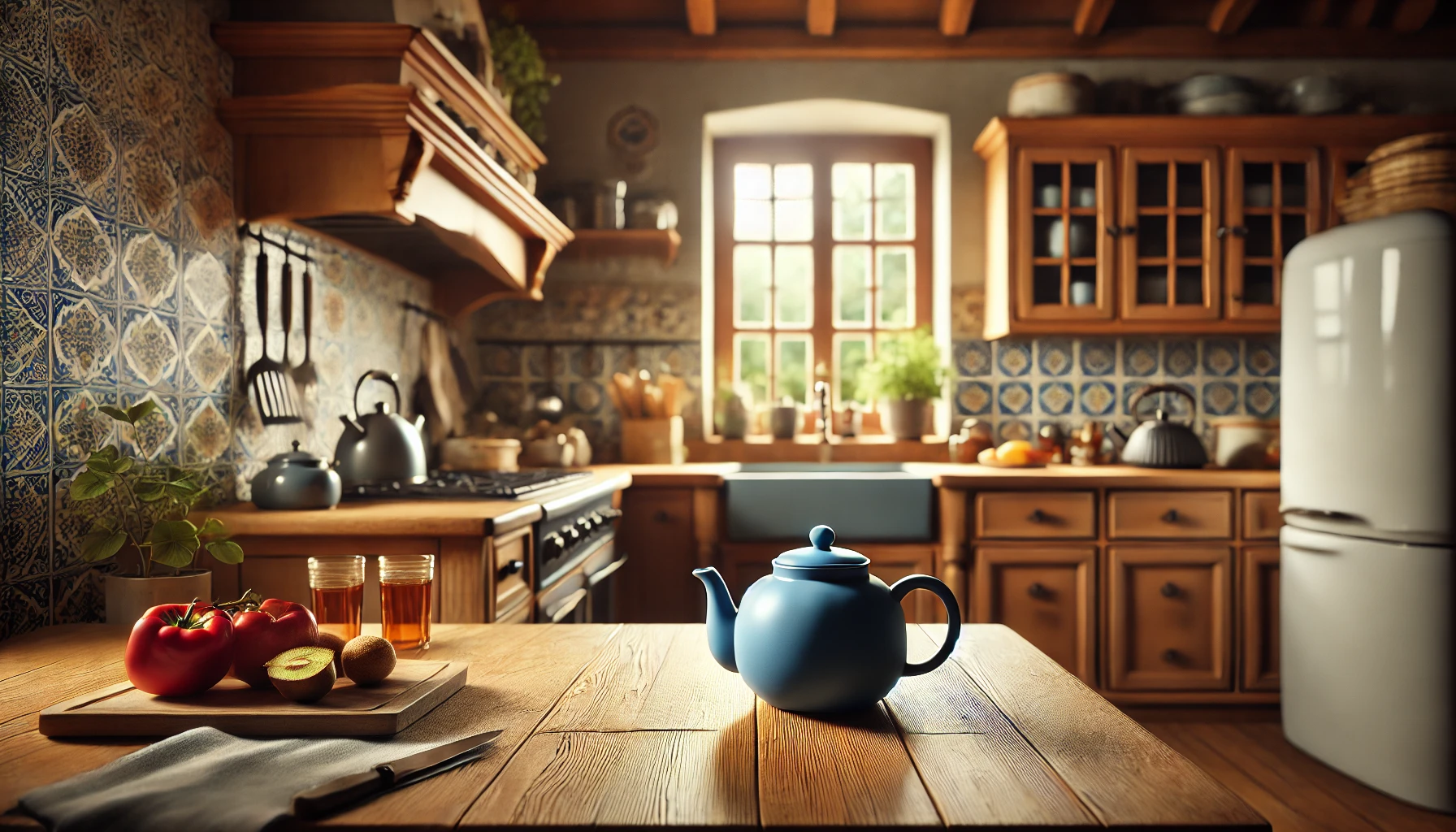
All product related images in this post were AI generated by OpenAI via ChatGPT. Benchmark images were manually created in Gimp Chart images were generated by matplotlib library in jupyter notebook