

This blog post was co-authored by Daniel Fatade, Sean Takafuji, Yana Valieva, and Nile Wilson. This deep dive is a follow-up to “Building an Action Detection Scoring Pipeline for Digital Dailies” by Samuel Mendenhall.
Introduction
While shooting a production, cameras are always on. The footage filmed for the entire day is called a “digital daily”. It includes multiple takes of scenes, as well as unnecessary transitional data. All those digital dailies are then permanently archived to cloud storage in high resolution, and up to 80% of their content is redundant. Obviously, this approach results in unnecessarily expensive storage costs.
Nowadays, archiving and later retrieval of digital dailies is a manual and time-consuming process. Archivists go through gigabytes of reels and identify which portions of content can be archived and/or discarded. Metadata of each scene and take is annotated manually as well. Together with WarnerMedia, the Microsoft Commercial Software Engineering (CSE) team developed a solution that can significantly reduce the time spent on this process by WarnerMedia’s archivists. While final review prior to deletion will have a ‘human in the loop’ editor, the automated prediction of discardable segments substantially reduces the time required.
We took advantage of well-known “action” and “cut” filming protocols. The content between “action” and “cut” should be kept, the rest of the content can be archived or discarded. To identify the “action” and “cut” events, we took the approach of identifying visual and audio cues present in the footage as a means of demarcating the portions of content with filmed scenes to be stored, and portions of non-scene and take footage that can be discarded.
Based on the source of the events that we needed to recognize, we identified the following workstreams:
- “Action” detection: we used clapperboards for their primary purpose, to identify the beginning of each take. We summed the problem up to binary classification of video frames: a model should automatically detect whether a picture contains a clapperboard or not.
- Metadata extraction: we managed to identify rolls, scenes, and several takes by using Optical Character Recognition (OCR) techniques for video frames, containing clapperboards.
- “Cut” detection: a clapperboard is not always presented at the end of a take, therefore we leveraged the video sound to recognize director commands. The end of a take is usually marked with a “cut” command. We used speech recognition techniques to transcribe the text and identify commands of interest.
Our solution heavily leverages Azure Machine Learning as the main experimentation platform, which allows us to run experiments on a remote low-cost compute in parallel mode, log metrics, and track model performance and version models.
Dataset
WarnerMedia provided 45-hour long footage of an action film that was divided into 191 files. We then empirically split the dataset into train, validation and test sets based on qualitative aspects of each video (e.g., green screens, dim lighting, rain, etc.). We elected to selectively sample per the above guidelines over a random sampling to ensure there was a representative sample over the distribution of different types of footage in all three sets. Thus, we produced the following datasets:
- Train set: 128 files, 31 hours of content.
- Validation set: 32 files, 7 hours of content.
- Test set: 31 files, 7 hours of content.
Frames extracted from this video dataset are referred to as the frame dataset.
“Action” Detection using Custom Vision
For clapperboard detection we took a Custom Vision experimentation path. This service allowed us to customize model training with the frames dataset, build a strong baseline for clapperboard recognition, and iterate the model to improve recognition quality. However, we had to cut through several obstacles, such as unlabeled data, imbalanced data, and systematic errors. In this section we explain the challenges we faced and demonstrate how we managed to overcome them.
Labeling
Labeled data is a strong requirement for the Custom Vision service. Our attempt at manual labeling cost us 40 minutes per video on average. Continuing with this method would result in approximately 18 working days for an 84k images subset, not even considering that it’s almost impossible to stare at the pictures more than 5 hours a day.
When we look deeper into the data, we notice one thing typical for this media data; there are lots of very similar images. How can we group these similar images and label these few groups instead of keeping all the frames extracted from each video?

In Figure 1 above, you can see our workflow. On the first step we have many unlabeled images. We then extract embeddings from these images using a commonly used lightweight VGG16 neural network, pretrained on the ImageNet dataset. After that, we feed them into the clustering algorithm. In our case we use the DBSCAN algorithm, which finds core samples of high density in a multi-dimensional workspace using a distance function and expands clusters.
For each video, we get a different small number of clusters and some of the noise points. Now we only need to manually assign labels to few clusters instead of to all the video frames. As a result, the time spent on labeling was reduced to 4-5 minutes per video, which resulted in needing only 2 working days for labeling.
Important to note, this method produces some false positives and false negatives because of its unsupervised nature. However, the noise level in the labels estimated by the algorithm is appropriate for training deep neural networks and did not have a negative impact on the final solution.
The code for the labeling tool has been operationalized as an Azure Search Power Skill and is available in the Azure-Samples repository.
Approach
Due to its nature, the frames dataset is highly imbalanced: the ratio between plain footage and footage containing clapperboards is skewed to the plain images (26:1). We decided to not proceed with standard balancing techniques such as randomly downsampling or upsampling the underrepresented class due to data loss and increased training time, respectively.
Instead, we decided to go ahead with our dataset-specific approach. Frames extracted from the media data are almost always excessive: an extraction frames per second (fps) of 1 allows you not to miss any scene changes, but also provides you with a lot of redundant, nearly identical, images that do not contribute to the model quality. Hence, we decided to reuse the clustering approach described in the labeling section for the plain images class. From each cluster, we selected 5 images (core point and nearest to them) and added all the noise points. This approach enabled us to get a 1.5:1 ratio of the classes in the frames dataset.
We also took the approach of data augmentation to address dataset imbalance. Even though Custom Vision provides some built-in augmentation techniques, the results of our experiments have shown that further augmentations might improve the model performance.
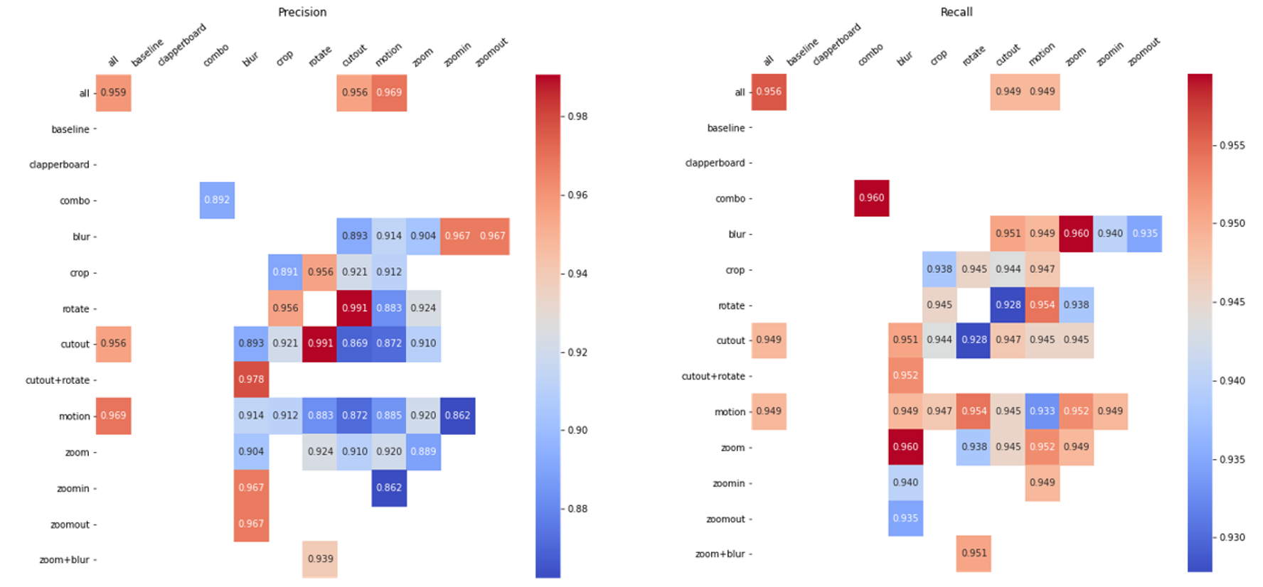
Inspired by the augmentation heatmaps approach described in the A Simple Framework for Contrastive Learning of Visual Representations paper (Chen et al., 2020), we decided to adopt this approach to systematically study the impact of different augmentation techniques on the model performance. We reproduced this approach with a specific set of augmentation that we found to be useful for our task based on the analysis of systematic errors. We consider several common types of augmentations here:
- Spatial/geometric transformation of data (e.g., crop, pad, rotate)
- Appearance transformation (e.g., blur, cutout)
- Color distortion (e.g., brightness, contract)
- Combo augmentations (a pipeline of augmentations applied to the same image)
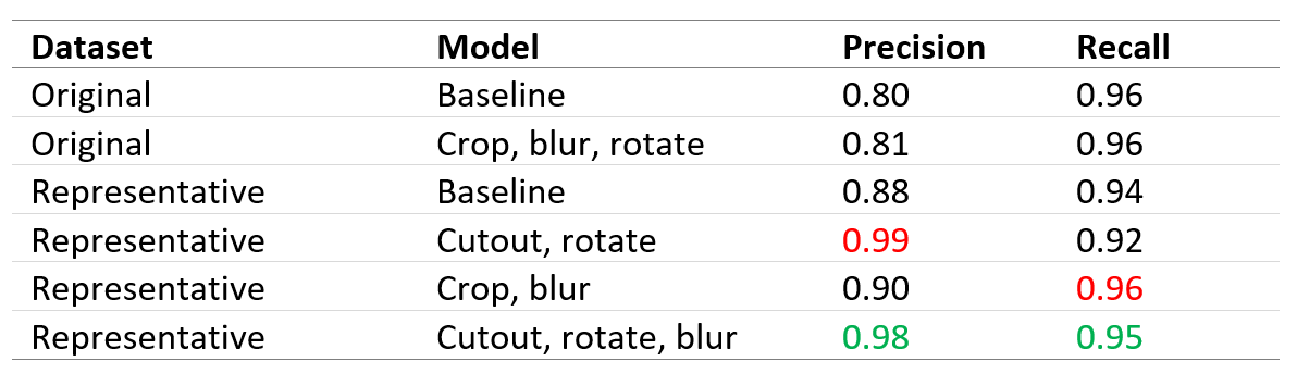
To understand the effects of individual data augmentations and augmentation composition, we investigated the performance of our framework by applying augmentations individually or in pairs using heatmaps provided below. Based on these heatmaps we managed to select a release candidate with the best tradeoff between important business metrics: precision and recall. Please, find the comparison of the models in the table above. Red color means best individual metrics, green one highlights the release model we have chosen.
Training Pipeline
We operationalized the Custom Vision training process by creating a reusable pipeline that consists of 4 steps. In the Image Augmentation Step, we applied the approach described in the previous section to generate an augmented dataset for further model training. This step takes a path to an augmentation configuration json file and saves the augmented dataset back to the Blob Storage. If the dataset that corresponds to the provided file already exists and no force flag is provided, the pipeline skips this step to spare computation time and resources.
The Custom Vision Training Step creates a new Custom Vision project and uploads the specified dataset to the Custom Vision service. Once the training is completed, we provide the Evaluation Step with the trained model information to validate the quality of the model. In this step, we calculate metrics for the newly trained Custom Vision model and log them to both Azure Machine Learning Studio and Application Insights. Using Azure Machine Learning Studio, Data Scientists and Machine Learning engineers can easily get detailed reports on model performance and track model improvements. For this purpose, we log model metrics, model architecture, augmentations applied, model training time, etc. For business users we built PowerBI dashboards with a limited number of metrics corresponding to the business objectives. These reports reflect changes in model performance over time.
Once the evaluation step is completed, we proceed to the Model Registration Step. This step is very important to ensure full model compatibility with the final solution scoring pipeline. Based on the artifacts produced by this step, the scoring pipeline will be able to fully reproduce the model and its parameters for further batch usage. To enable this compatibility, we save the following artifacts as a model to the model registry:
- The model itself. In this case, a model is represented by a .json file containing all the required properties to choose the right Custom Vision project and iteration (project name, iteration id).
- A .csv file containing the description of a dataset the model was trained on.
- A .json augmentation configuration file for a full reproduction of the dataset the model was trained on.
- A .csv file containing lists of False Positives, False Negatives for further systematic errors analysis.
- Hyperparameters of the model as registered model tags.
All these artifacts guarantee full compatibility between the training pipeline and our final solution scoring pipeline.
Clapperboard Metadata Extraction using Azure Form Recognizer
Another key aspect of the solution was to effectively find a means of extracting text-based metadata from clapperboard images at scale in order to identify rolls, scenes, and takes. In order to effectively extract metadata from many clapperboard images at scale, we utilized an MLOps solution which consisted of a series of steps:
- Azure Custom Vision Step: Predict Clapperboard Images (as described in the previous section).
- Clapperboard Selection Step: Select the most “informative” image from a batch of clapperboard images using Optical Character Recognition (OCR).
- Azure Form Recognizer Step: Run OCR on selected images and produce key-value pairs for predicted text elements.
- Postprocessing Step: Use a rule-based approach to improve results from the Azure Form Recognizer
An illustration giving an overview of the vision portion of the solution is provided below:

Challenges
Initially, our research led us to believe that the Azure Form Recognizer Cognitive Service would be sufficient to automate the process of extracting text and generating key-value pairs for clapperboard items such as roll, scene, take and more. However, after some experimentation, we realized that the default service was unable to meaningfully extract and map any values of interest. This was not unexpected given that the default model was trained to generalize as much as possible, specifically for key-value extraction with business cards, receipts and more.
Nonetheless, we believed the service could still be of use given a custom approach. This led to the idea of training a custom model in Azure Form Recognizer Service by utilizing a representative sample of our clapperboard dataset. However, the cost of training and utilizing a custom model in Azure Form Recognizer service can be rather steep.
The cost of running predictions on the custom service would amount to $50 per 1000 images. In comparison, the default service cost $10 per 1000 images processed. Given that we anticipate the service will process possibly millions of clapperboard images, it was imperative that we found a means to minimize cost. This is what led to the hypothesis of using the Azure Cognitive Services Computer Vision Read API (OCR) and a character-level frequency scoring function to select the most informative image from a set of similar images.
Approach
For this workstream, we utilized OCR technology that was made available through the Azure Cognitive Services Computer Vision Read API. This technology was trained to interpret both handwritten and printed text. This was useful for metadata extraction given that the clapperboard images we worked with generally contained a mix of both printed and handwritten text. Generally, each of the video files contained a set of “action” events. Within each action event, we were provided with a set of clapperboard images, in which each of the images were visually similar to one another. We identified three possible types of images within each event:
- A blurry clapperboard image, where the clapperboard object is being brought into the frame.
- A still clapperboard image, where the image has successfully been brought into the frame.
- A blurry clapperboard image, where the clapperboard object is being taken out of the frame.
From our findings, the blurry clapperboard images did not offer much value, given that the OCR service could barely detect any text within these images. The only meaningful image types were the still clapperboard images. As you can imagine, when extracting image frames from video, there will be multiple duplicate or similar frames depending on the number of frames extracted per second. In our case, we extracted one image frame per second (1 fps), as these were the input parameters specified to the Custom Vision step (please refer to the Custom Vision section for an explanation regarding clapperboard detection and the decision to use 1 fps for frame extraction purposes) With this, we identified that for each action event, there was at least more than one still image.
Given that each still image in a respective action event essentially contains the same metadata we wish to extract from clapperboards, we decided to utilize only one of these images per action event. This presented the challenge of knowing how to select the best or the most informative clapperboard for each event, where the most informative clapperboard image is the image where the OCR model can extract the most meaningful text from.
Since we were relying heavily on OCR for this workstream, we decided it would be a good approach to utilize a character-level frequency function to score and identify the most informative image. The idea is that the image with the most predictable text will have the highest character count. Thus, the image with the highest character count will be identified as the most informative.
Conveniently, the OCR service was at a lower cost when compared to using a custom model in Azure Form Recognizer (around $2.50 per 1000 images processed for standard pricing). Given this, we could afford to feed in millions of images into the service and filter out unnecessary images before sending results to the custom model in the Azure Form Recognizer cognitive service.
Labeling
As mentioned earlier, utilizing a custom model in Azure Form Recognizer is expensive. However, by utilizing the clapperboard selection step, we can significantly reduce the costs incurred by the custom service given that only a subset of clapperboard images are fed into the model. In order to train a custom service, we aimed to:
- Select and make use of a representative set of clapperboard images to be used in training the custom model.
- Utilize the Azure Form Recognizer sample-labeling tool to tag text artefacts from the representative dataset with appropriate labels.
- Train a custom model in Azure Form Recognizer using a set of asset files generated from the sample labeling too
- Package the entire training process as a series of steps to be run within an Azure Machine Learning (AML)
As described earlier in the Custom Vision workstream section, we implemented a density-based clustering algorithm to generate a representative sample of our clapperboard dataset. This representative dataset was then used within the Azure Form Recognizer sample labeling tool.
The Azure Form Recognizer sample labeling tool is an application that provides a simple user interface, which we can use to manually label forms (documents or images) for the purpose of supervised learning. The tool reads in a set of documents or images from a specified blob storage container. From here, we can run OCR on all the read-in content and assign labels to predicted text artefacts. These set of labels can then be used to train a custom model in Azure Form Recognizer.
Generally, the average clapperboard contains the following items:
- Roll – The roll of film stock used for the current take.
- Scene – The ID of the scene that is currently being shot/filmed.
- Take – The current take number for a particular scene.
- Director– Director of the project.
- Co-director/camera – Co-director or the individual who filmed the scene.
- Title– The title of the project. In this case, the title could be the name of your favorite movie, let’s say for example, “The Dark Knight”.
- Description – Extra text/information describing a particular scene in some cases.
A set of asset files are required to effectively train the service. For each image, we need the following:
- An ocr.json file that contains information regarding all predicted text items and bounding boxes generated on a single image/document.
{
    "status": "succeeded",
    "createdDateTime": "2021-03-01T19:19:35Z",
    "lastUpdatedDateTime": "2021-03-01T19:19:40Z",
    "analyzeResult": {
        "version": "2.0.0",
        "readResults": [
            {
                "page": 1,
                "angle": 0.6682,
                "width": 5398,
                "height": 3648,
                "unit": "pixel",
                "language": "en",
                "lines": [
                    {
                        "boundingBox": [ 3843, 1485, 3798, 1348, 3832, 1337, 3879, 1473],
                        "text": "dry erase",
                        "words": [
                            {
                                "boundingBox": [...],
                                "text": "dry",
                                "confidence": 0.648
                            },
                            {...}
                        ]
                    }
                ]
            }
        ]
    }
}
- A labels.json file containing information regarding assigned labels to predicted text artifacts within a single image/document.
{
    "document": "image_1.jpg",
    "labels": [
        {
            "label": "roll",
            "key": null,
            "value": [
                {
                    "page": 1,
                    "text": "01",
                    "boundingBoxes": [
                        [0.3356, 0.4564, 0.3884, 0.4547, 0.3892, 0.5032, 0.3366, 0.5052]
                    ]
                },
                {
                    "page": 1,
                    "text": "A",
                    "boundingBoxes": [
                        [0.3021, 0.4665, 0.3147, 0.4665, 0.3142, 0.4942, 0.3017, 0.4939]
                    ]
                }
            ]
        },
        {
            "label": "title",
            ...
        }
    ]
}
In total, to successfully train a custom model in Azure Form Recognizer service, we need the original image file, an ocr.json file and a labels.json file (examples shown above). These two asset files can be rather large and tricky to fill in manually. Luckily, the sample labeling tool automatically generates these asset files and stores them within the same storage container the images were read from. This means that once labeled, as long as a SAS URI pointing to the container is made available, the process of training the model can be automated by utilizing a Python script within an AML pipeline.
Character-Level Frequency Scoring
We managed to achieve an average accuracy of around 80% across all classes, with the addition of a postprocessing step, by utilizing a small sample of around 300 clapperboard images. This implies that a relatively small dataset can be used to achieve fairly good results.
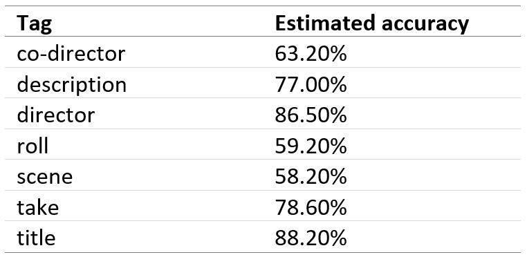
One thing to note is that the Azure Form Recognizer uses the same OCR technology as the Azure Cognitive Services Computer Vision Read API. As a result, any predictions the OCR service fails to make will be reflected in the results of the custom model trained with Azure Form Recognizer service; i.e, if the OCR fails to pick up a “scene” item, the Azure Form Recognizer service will output and empty key-value pair for “scene”.
End of Scene Detection using Custom Speech from Azure Cognitive Services
A key aspect of the solution is to note where the end of a scene occurs. In a majority of cases, the only indication of the end of a scene is an utterance of the word “cut’ by the director. As a result this requires a speech recognition solution to detect this keyword. Our baseline model was the “out-of-the-box” variant of Speech to Text from Azure Cognitive Services. Our initial assessment was that Speech to Text was producing too many false negatives, resulting in low recall scores and leading us to experiment with custom modeling approaches. The custom modeling approaches we experimented with were an adoption of FixMatch for the audio space, VGGish Embeddings trained on the benchmark dataset Youtube-8M, and Speech Embeddings trained on the benchmark dataset Speech Commands. Of the three approaches, Speech Embeddings had the best performance metrics for our task.
Within the training pipeline of our final solution, we utilize Custom Speech from Azure Cognitive Services for the task of detecting “cut” utterances.
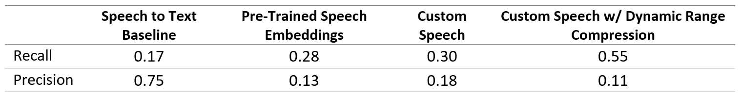
In Table 3, we note the key milestones where an improvement to the audio aspect of the solution was made. Note that Table 3 refers to the metrics regarding “cut” detection while our final business metrics are for the task of identifying portions of footage “to archive” or “to discard”. To increase our final business metrics, it is desirable to prioritize having a higher recall even if it means a loss of precision and a reduction of our overall f1-score. This is due to the following outcomes of postprocessing:
- Multiple false positive “cuts” can be reduced by grouping predictions to each other that are nearby in time.
- A false positive “cut” that occurs between a true positive “action” and “cut” is completely ignored as we will mark the entire section as “to archive”.
As a result of the above postprocessing steps, the final business metrics on the classification of footage “to archive” and “to discard” has performance metrics of 0.96 precision and recall.
Challenges
The key challenges with the audio detection of the utterance of “cut” were due to the nature of the microphone capture.
- Challenge #1: No Transcription Provided. The provided videos were not equipped with an accompanied transcription nor information on key timestamps where a scene began and ended. As a result, to treat this as a supervised classification problem, we would first need to undergo a manual labeling process to build a training set.
- Challenge #2: Distant Speaker. The primary microphone capture for the footage we worked with is for the actors and the environmental sounds within a scene. As a result, the director and their crew were always a secondary capture, comparable to background speakers. Thus, our speech recognition task focused on correctly identifying when a soft and distant speaker uttered the word “cut”.
Labeling
To address Challenge #1: No Transcription Provided, we underwent a manual labeling effort throughout the lifetime of the project, with labels “action-utterance-action” and “cut-utterance-cut”.
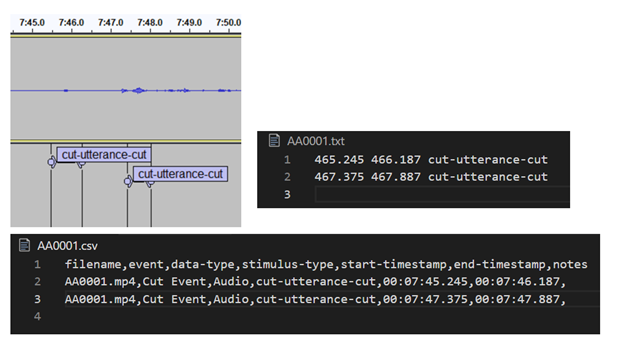
To gain a precise start and end timestamp we utilized a tool called Audacity®, which is an open-source and cross-platform audio editor. When opening a file in Audacity®, we can add labels to a label track as seen in Figure 4. Per our label schema, whenever a “cut” that indicated the end of a scene was uttered, we would add the label “cut-utterance-cut”. All the labels on the label track can then be exported as a txt file which is then converted to a csv format during the preprocessing step of the training pipeline. The label files are than aggregated for the files in the train, validation, and test sets.
Dynamic Range Compression
The preprocessing step also addresses Challenge #2: Distant Speaker through the usage of dynamic range compression. Dynamic range compression is an audio signal processing operation that reduces the difference between the smallest and largest value in the signal, reducing the volume of louder noises while increasing softer ones. This brings the director and film crew’s utterances of “cut” that were soft and, in some cases, nearly inaudible close to the forefront of the audio signal.
for step in step_order:
    t_start_step = datetime.now()

    output_audio_dir = join(output_audio_dir, step)
    input_audio_filepath = output_audio_filepath
    output_audio_filepath = join(output_audio_dir, audio_filename)

    # Dynamic Range Compression
    if step == "compress":
        run_ffpmeg_dynaudnorm(
            input_audio_filepath, output_audio_filepath, overwrite=overwrite
        )

    # Denoising
    elif step == "denoise":
        denoise_audio(
            input_audio_filepath,
            output_audio_filepath,
            overwrite=overwrite
        )
    # Format Audio for Custom Speech Service
    elif step == "reformat":
        reformat_audio_for_custom_speech(
            input_audio_filepath, output_audio_filepath, overwrite=overwrite
        )
    runtime[step] += (datetime.now() - t_start_step).total_seconds()
The above code block shows a preprocessing loop. To allow flexibility with the order of these preprocessing steps during experimentation, the step_order is defined as a list such as [“denoise”, “compress”, “reformat”] and the functions will be applied in that order. More information about Dynamic Range Compression available in the ffmpeg documentation.
Formatting the Training Dataset for Custom Speech
After reformatting the audio files per Custom Speech requirements, the training dataset requires additional handling via extracting only the segments captured in the bounding box labels. These segments are written out as individual 2 second duration wav files with the pattern {filename}-{word}-{id}.wav. If the bounding box was for less than 2 seconds, the waveform is right padded with zeroes. To reduce the number of false positives, we additionally added samples of similar sounding words such as “but” and “cat” alongside the “cut” audio samples. Accompanying these files is a single transcription file, Trans.txt, where each line is the filename followed by a machine-friendly English transcription of the words spoken in the file. The segments and transcription file are written out to a single directory which is then archived to be uploaded to Custom Speech’s datasets.
Training and Evaluation
To utilize Custom Speech, we leveraged the Python Swagger SDK variant to make API calls.
For the AML step “train_and_evaluate” in the following intermediate steps occur:
- The training and validation datasets are registered on Custom Speech.
- A baseline Speech to Text model is selected to finetune based on our training data.
- The model undergoes training.
- The model transcribes each wav file in the validation dataset.
- The transcriptions for each wav file are retrieved from Custom Speech and parsed for any detection of “cut”.
- The classification metrics are computed and aggregated across all files in the validation dataset.
- The classification metrics, dataset IDs, and model ID are logged to the AML experiment.
- Through the Azure DevOps pipeline that triggers the AML pipeline, a newly trained model can be marked as the one for production.
Selecting the Baseline Speech to Text Model
When training a Custom Speech model, a Speech to Text model is used as the initial baseline to train from. Whenever the training pipeline runs, the newest available model is always utilized. As the mechanism to mark a model for production requires human approval, this automatic change would only be released if a data scientist marks the model for use in the final solution scoring pipeline.
Evaluation on the Validation Dataset
When custom speech evaluates an audio file, it creates a JSON transcription (as seen below). For each entry in recognized phrases, we parse the results in “nBest” followed by each word in “words” to determine if a “cut” was detected in the transcription. For clearer insight at this stage of the evaluation, we do not factor in the confidence score of “cut” when comparing the predictions against the ground truth.
{
    "source": "test_1.wav",
    "timestamp": "2020-09-18T12:29:49Z",
    "durationInTicks": 6120600000,
    "duration": "PT10M12.065",
    "recognizedPhrases": [
        {
            "recognitionStatus": "Success",
            "channel": 0,
            "offsetInTicks": 100000000.0,
            "durationInTicks": 120000000.0,
            "nBest": [
                {
                    "confidence": 0.53361744,
                    "lexical": "cut",
                    "itn": "cut",
                    "maskedITN": "",
                    "display": "cut",
                    "words": [
                        {
                            "word": "cut",
                            "offset": "PT1.54S",
                            "duration": "PT0.23S",
                            "offsetInTicks": 15400000.0,
                            "durationInTicks": 2300000.0,
                            "confidence": 0.53361744
                        }
                    ]
                }
            ]
        }
    ]
}
The above code block shows an example transcription created by Custom Speech on a validation / scoring wav file input.
Metrics Calculation
For the classification metrics, when comparing the predictions against the ground truth we allow the timestamps to differ by an amount “ts_threshold”. This allows a slight discrepancy in the timestamp of detection from the transcription and our ground truth label to still be classified as a true positive. In our reported metrics, we used a “ts_threshold” value of 3 seconds meaning a detected “cut” can differ from the ground truth timestamp by +/- 3 seconds. Ultimately, as detecting “cut” is an auxiliary task for finding the ending timestamp of a scene, being a few seconds off has a negligible effect as it is expected the “to archive” section will retain a few seconds before and after the precise scene.
Final Solution: The Scoring Pipeline
Our final solution consolidates the “action” event detection, clapperboard metadata extraction, and “cut” utterance detection work into a multi-model batch scoring pipeline deployed through Azure Machine Learning. In Figure 5, we see a representation of the full scoring pipeline which includes the previously described workstreams, as well as a report compilation step which will be discussed further in this section.
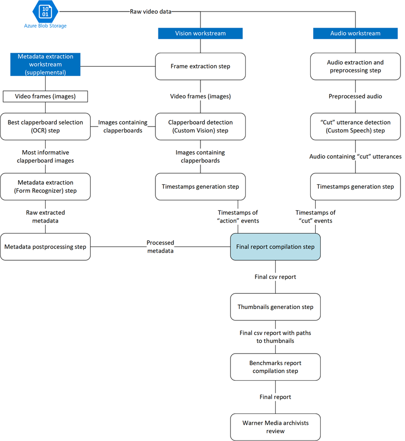
The raw video data is passed from Azure Blob Storage into the vision and audio workstreams in parallel. The metadata extraction workstream relies on output from the vision workstream whereas the audio workstream acts independently. Once these three workstreams are complete, a final report compilation step is triggered. This final report builds upon the outputs from the vision, metadata extraction, and audio workstreams to provide timestamp ranges of “to archive” and “to discard” footage from the input video.
In the following subsections, we tie together each workstream’s contribution to the final solution.
Vision Workstream
In the vision workstream, the first step is the Frame Extraction Step. We use ffmpeg (fps = 1) and the same augmentation methods applied with the registered model during training parameters here that we carefully logged in the model registration step.
Like in the training pipeline, we have a Custom Vision Step here that is used to predict whether the pictures extracted by the previous step contain a clapperboard or not.
The Timestamp generation Step here requires additional attention as it is not enough to only get binary labels for the pictures extracted from the videos. We also produce “action” event timestamps. In fact, each picture represents one second of the video. Therefore, we get a sequence of seconds labeled with “plain” and “clapperboard” timestamps. For this purpose, we merge all the detected neighboring clapperboards into one event with the tolerance of 2 seconds. For example:
- “clapperboard, clapperboard, clapperboard” sequence will result in one “action” event with the first detected clapperboard timestamp marked as the resulting timestamp.
- “clapperboard, plain, clapperboard” sequence will result in one “action” event with the first detected clapperboard timestamp marked as the resulting timestamp, as we have a tolerance of 2 seconds defined.
- “clapperboard, plain, plain, clapperboard” sequence will result in two “action” events with the first detected clapperboard timestamp marked as the resulting timestamps respectively.
Once the timestamps are ready, we feed them into the Final Report Compilation step to merge them with the events detected by the other workstreams.
Metadata Extraction
Once the vision workstream custom vision step completes, the metadata extraction workstream begins. This workstream extracts relevant metadata from the detected clapperboards, such as scene and take.
As described in the vision workstream, clapperboards appear in the footage in a series of consecutive frames, leading to redundant images. By utilizing OCR to select the best clapperboard, we were able to:
- Reduce the number of calls made to the Azure Form Recognizer cognitive service by 73%, effectively reducing the cost of utilizing the service.
- Reduce the time spent on predictions as we were feeding in less images to the cognitive service.
- Reduce time spent on proceeding steps that were dependent on the Azure Form Recognizer step since they were processing less files.
Utilizing OCR and a character-level frequency scoring function played a key role in the cost optimization for our operationalized multi-model service. In the context of WarnerMedia, the implementation of clapperboard selection allows them to effectively minimize cost as much as possible while delivering on their business needs. We have high confidence that this pairing can be utilized across a multitude of reels where we expect to see a large number and variety of clapperboard images.
Audio Workstream
In tandem with the vision workstream, the raw video data from Azure Blob Storage is passed into the audio workstream. The first step is to extract and process the audio in the same fashion as in the training pipeline for “cut” utterance detection.
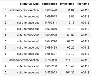
Like for the other workstreams, the scoring pipeline retrieves the latest – in this case, audio – model from the AML model registry with the tag “status: production”. The scoring pipeline then generates a csv of predictions as seen in Figure 6.
The “cut” utterance timestamps are then fed into the report compilation step to help identify the ends of takes, ultimately assisting in identifying portions of film as “to archive” or “to discard”.
Archival and Performance Report Generation
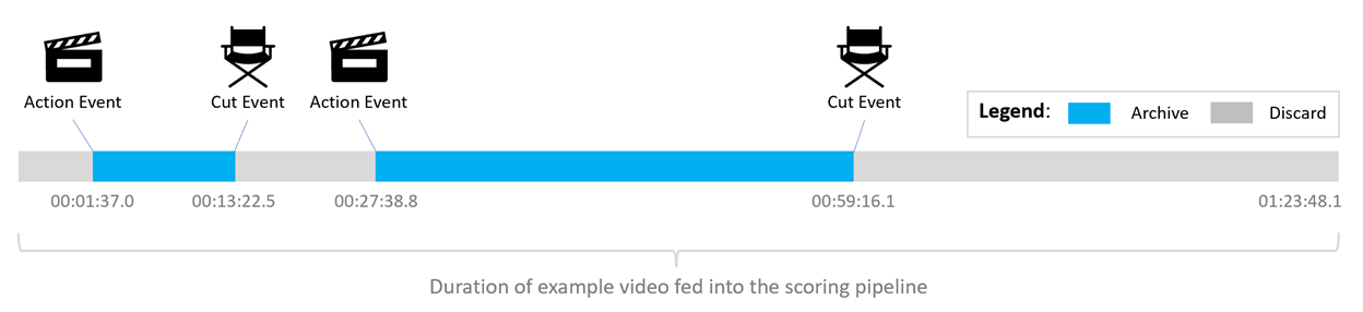
With the custom vision, metadata extraction, and audio workstreams complete, the final report compilation step can begin. This step consolidates the “action” event timestamps provided from the vision workstream and “cut” event timestamps provided from the audio workstream to identify portions of the input video as “to archive” or “to discard” (see Figure 7).
The timestamps and labels for each input video are organized into a single final report json file. Following this, three thumbnails are generated for each detected “action” event to allow for easy review.
In the below section, we go into detail on the benchmarks report compilation step.
Benchmark Report Compilation
One of the key objectives was to improve observability regarding pipeline performance and to automatically log metrics useful for cost estimation into a single, convenient report. This insight into compute costs and potential storage cost savings empowers business executives to make informed decisions regarding the archiving process.
The PipelineBenchmarker is a lightweight and generalizable framework that enables automatic logging of metrics relevant to pipeline performance evaluation. While existing tools built-in to Azure Machine Learning enable ML model metric tracing, this framework focuses on metrics relevant to resource decision making.

By tracking values such as compute configuration (e.g., compute target name tied to specific AML cluster size and type), number of nodes used, and the time to complete each step and the total pipeline, we gained a clear understanding of (1) what steps are the most computationally heavy and (2) what parameters and compute configurations could be optimized for either cost or speed.
Azure Cognitive Services Consumption
In addition to basic compute configuration and duration benchmarks, we were interested in logging Azure Cognitive Services consumption throughout our solution pipeline for cost estimation. As described above, the final scoring pipeline solution consists of an audio workstream which calls the Custom Speech service and a vision workstream which calls the Custom Vision, OCR, and Form Recognizer services.
These Cognitive Services consumption metrics written to the final benchmark report provide the customer with an understanding of approximate cost and allow them to estimate future costs. This also allows them to break down the costs by service called, which is helpful in cases like ours where one service (i.e., Form Recognizer) is notably more expensive.
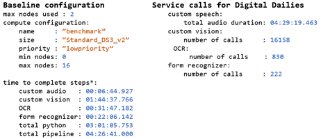
Figure 9 below displays the total number of hours spent running the entire MLOps solution. In the figure, you will notice that the number of API calls made to the Azure Form Recognizer are significantly much less than the number of calls made to the OCR service. Furthermore, time spent running the Azure Form Recognizer step was less than that of the Clapperboard Selection step (OCR step). This was a great improvement given that on average, the custom model trained in Azure Form Recognizer takes around 3 or 4 times longer than the Azure Cognitive Services Computer Vision Read API to process an image file.
Labeling Production Footage for Discard
Building upon the basic pipeline benchmarking framework, we also log data addressing our main goal of identifying discardable footage.
The input to the pipeline is a directory of video files which are then split into audio and images by the pipeline to extract scenes, beginning with clapperboard image detection for “action” and ending with “cut” utterances from the director.
We modify the benchmark report generation step such that the resultant report structure separates individual video metrics from aggregate metrics. For any individual video, information such as what percentage or duration to archive or discard is included alongside the path to a detailed report file containing the specific timestamps for these archive/discard labels.
Impact of the Benchmarking Framework
This framework allows the user to easily evaluate the effect of compute configuration on step and whole pipeline duration, as well as log information relevant to cost estimation, including but not limited to Azure Cognitive Services consumption and storage costs.
With the generated benchmark report, WarnerMedia was able to estimate potential storage cost savings of implementing this multi-model ML solution in labeling portions of production footage to review for discard.
Conclusion
In partnership with WarnerMedia, we developed an operationalized multi-model approach to identify discardable portions of digital dailies, at scale, to assist archivists in processing large reels of footage. Our solution utilizes various Azure Cognitive Services as well as custom code executed in the Azure Machine Learning platform to identify and label segments of digital dailies as “to archive” or “to discard” as part of a comprehensive scoring pipeline.
While these models were trained and tested on the digital dailies provided to us, the solution itself is a generalizable approach and may aid in archiving efforts for many more films under WarnerMedia.
Ultimately, our scoring pipeline was able to identify over an hour of discardable footage in the provided reel using the combined custom vision and audio approach, leading to a 44% reduction in the archival storage cost. Here, we have demonstrated that this Machine Learning-powered and automated approach can aid archivists in efficiently processing digital dailies while preserving footage of interest for any given film.
Acknowledgements
Thank you to everyone involved in this collaboration between Microsoft CSE and WarnerMedia. Special thanks to Michael Green and David Sugg from WarnerMedia.
Contributors to the solution from the Microsoft team listed in alphabetical order by last name: Sergii Baidachnyi, Andy Beach, Kristen DeVore, Daniel Fatade, Geisa Faustino, Moumita Ghosh, Vlad Kolesnikov, Bryan Leighton, Vito Flavio Lorusso, Patty Ryan, Samuel Mendenhall, Simon Powell, Sean Takafuji, Yana Valieva, and Nile Wilson.