
I do believe this is great news for the ML.NET community and .NET in general. You can now run .NET code (C# / F#) in Jupyter notebooks and therefore run ML.NET code in it as well! – Under the covers, this is enabled by ‘dotnet-try’ and its related .NET kernel for Jupyter (as early previews).
The Jupyter Notebook is an open-source web application that allows you to create and share documents that contain live code, equations, visualizations and narrative text.
In terms of ML.NET this is awesome for many scenarios like data exploration, data cleaning, plotting data charts, documenting model experiments, learning scenarios such as courses or hands-on-labs, quizzes, etc.
Show me the code and run it!
Although I’m showing in the following steps most of the code, step by step, it is always useful, especially when dealing with Jupyter notebooks to have the Jupyter notebook code and simply run it!
I set up a Jupyter environment in MyBinder (public service in the Internet) which is a great way to try notebooks if you don’t have Jupyter setup in your own machine. You can run it by simply clicking on the below link:
Ready-to-run ML.NET Jupyter notebook at MyBinder
In that ready-to-run Jupyter notebook you can directly try ML.NET code, plotting charts from C#, display the training time and quality metrics, etc. as shown in the image below:
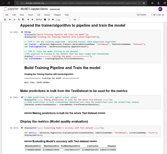
You can also download the Jupyter notebook with ML.NET code that I’m using in this Blog Post from here (MLNET-Jupyter-Demo.ipynb).
Note that after some time if your MyBinder environment was not active, it’ll be shutdown. Therefore, if you want to have a stable environment you might want to set it up on your own machine, as explained below.
Setting it up on your local machine
If you want to set it up on your local machine/PC, you need to install:
- Jupyter (Easiest way is to install Anaconda).
- ‘dotnet try’ global tool.
- Enable the .NET kernel for Jupyter.
Install Jupyter on your machine
The easiest and recommended way to install Jupyter notebooks is by installing Anaconda (conda) but you can also use pip.
When installing anaconda, it’ll also install Python. However, I want to highlight that ML.NET doesn’t have any dependency on Python, but Jupyter has.
For more details on how to install Anaconda and Jupyter please checkout the Jupyter installation guide.
Install the ‘dotnet try’ tool
The Jupyter kernel for .NET is based on the ‘dotnet try’ tool you need to install first.
The ‘dotnet try’ tool is a CLI Global Tool so you install it with the ‘dotnet CLI’.
Since these versions are early previews, they are still not in NuGet.org but in MyGet, therefore you need to provide the MyGet feed, like in the following CLI line:
dotnet tool install -g dotnet-try
Note: If you have the dotnet try global tool already installed, you will need to uninstall before grabbing the kernel enabled version of the dotnet try global tool.
List what Global Tools you have installed:
dotnet tool list -g
Update dotnet-try:
dotnet tool update -g dotnet-try
Uninstall:
dotnet tool uninstall dotnet-try -g
Issues and Open Source code
The ‘dotnet try’ tool open source repo is here: https://github.com/dotnet/try . You can research there for deeper details about it.
Issues and Feedback: If you have any issue with dotnet-try or the .NET kernel on Jupyter, please post it here: https://github.com/dotnet/try/issues
Install the .NET kernel in Jupyter
- If you have Jupyter using Anaconda then you should execute the commands below inside the Anaconda command prompt
- Run the following command
dotnet try jupyter install
- Run the following command

Test that it is working
-
- Start the Anaconda Navigator app (Double click on ‘Anaconda Navigator’ icon)
- Launch Jupyter from the ‘Launch’ button in the ‘Jupyter Notebook’ tile.
- Alternatively, from the Anaconda Prompt you can also start Jupyter by typing the following command positioned at your user’s home path.:
jupyter notebook
- You will see Jupyter and your User’s folders by default.
- Open the ‘New’ menu option and you should see the ‘.NET (C#)’ and ‘.NET (F#)’ menu options:

- Select ‘.NET (C#)’ and start hacking in C# in a new Jupyter notebook! 🙂
- For instance, you can test that C# is working with simple code like the following:

Ok, let’s hack for a while and start writing ML.NET C# code in a Jupyter notebook! 🙂
Install NuGet packages in your notebook
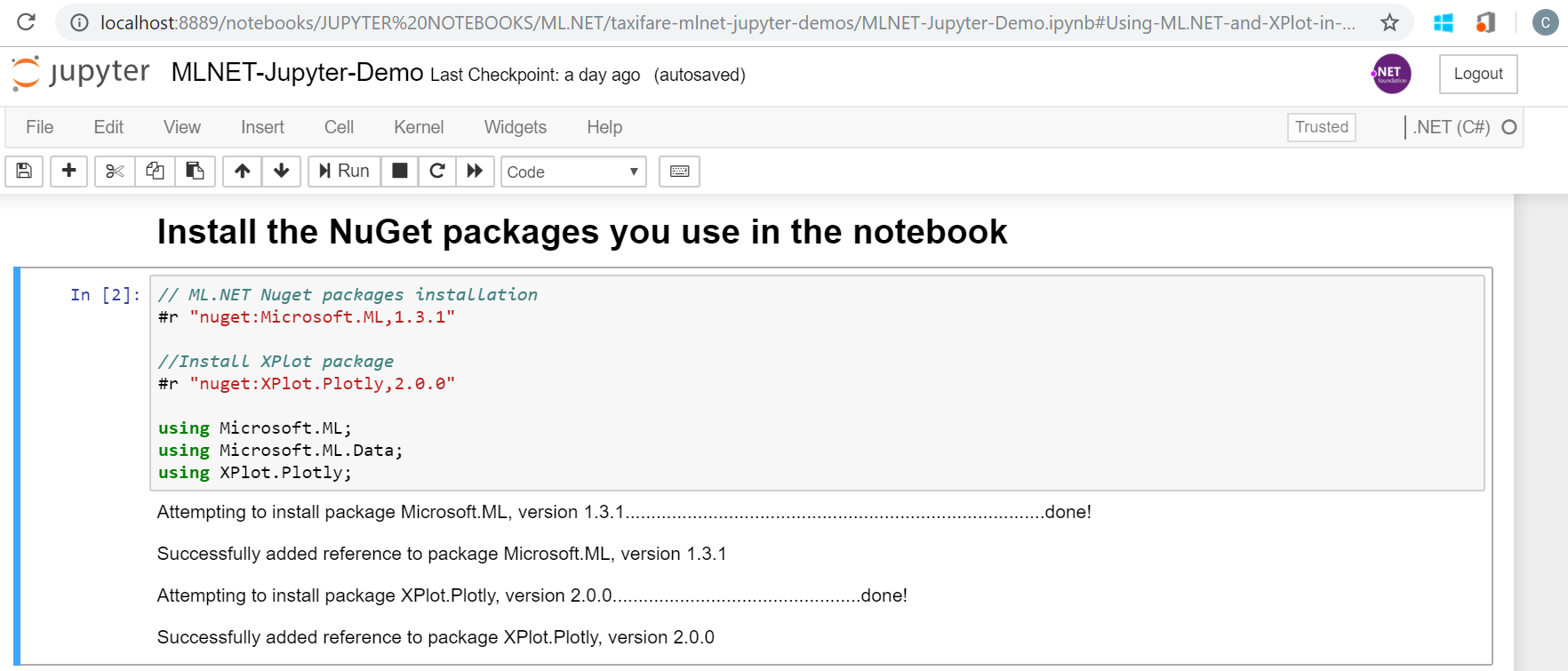
First things first. Before writing any ML.NET code you need the notebook to have access to the NuGet packages you are going to use. In this case, we’re going to use ML.NET and XPlot for plotting data distribution and the regression chart once the ML model is built.
For that, write code like the following. Versions might vary and you could also add the ‘using’ namespaces later on or in this same Jupyter cell:
// ML.NET Nuget packages installation
#r "nuget:Microsoft.ML,1.3.1"

//Install XPlot package
#r "nuget:XPlot.Plotly,2.0.0"
Run this cell once. It ‘ll take some time in order to download and install the NuGet packages, that’s why it is a good idea to have this installation in a separated cell.
Declare the data-classes
When loading the datasets and when training or predicting you need to use an input class and a prediction class, like the following classes:
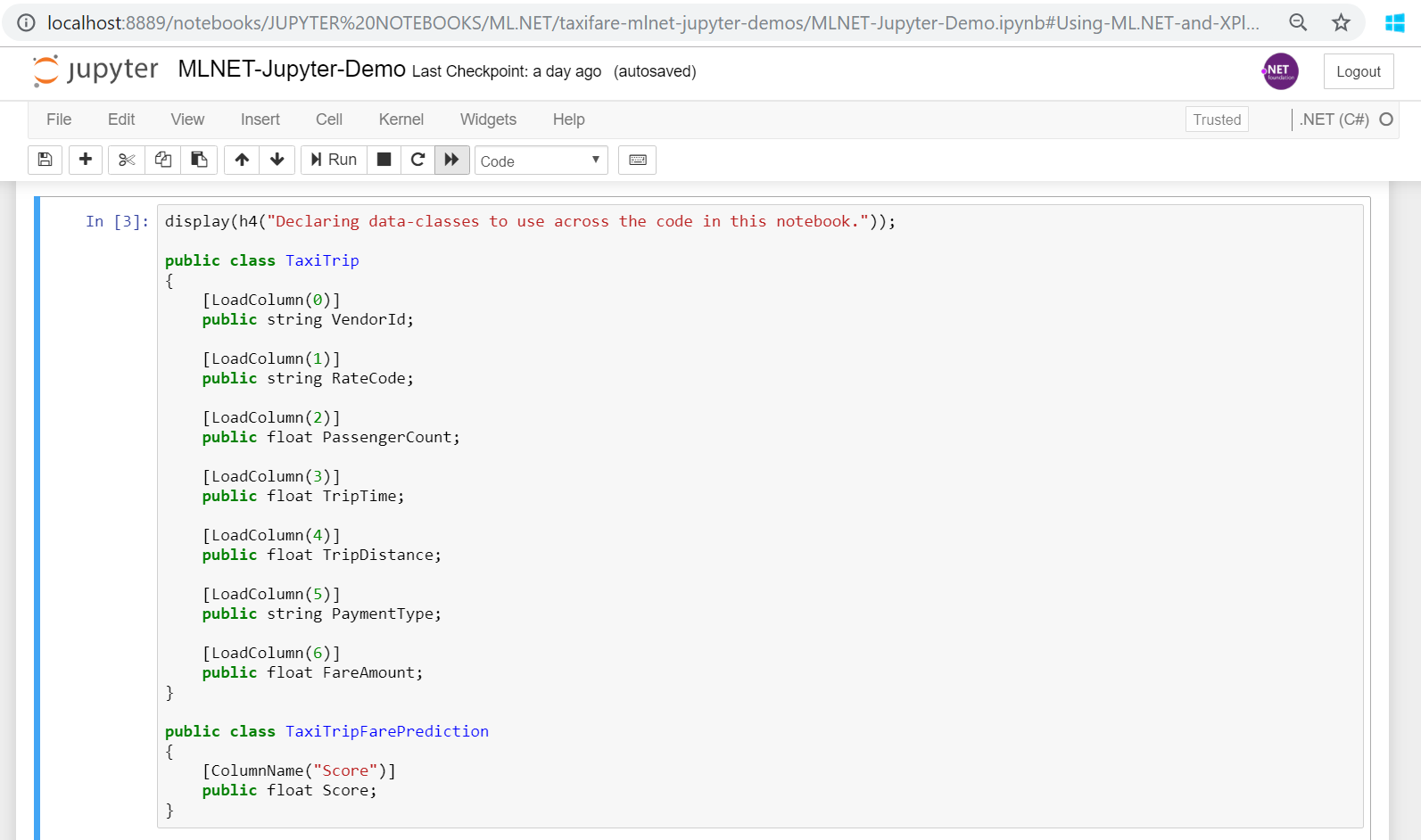
Here’s the code you can copy/paste in your notebook:
public class TaxiTrip
{
[LoadColumn(0)]
public string VendorId;

[LoadColumn(1)]
public string RateCode;

[LoadColumn(2)]
public float PassengerCount;

[LoadColumn(3)]
public float TripTime;

[LoadColumn(4)]
public float TripDistance;

[LoadColumn(5)]
public string PaymentType;

[LoadColumn(6)]
public float FareAmount;
}

public class TaxiTripFarePrediction
{
[ColumnName("Score")]
public float Score;
}
Load dataset in IDataView
The way you load data is exactly the same way you’d do in a regular C# project. You only need to place the dataset files in the same folder where you have your just created Jupyter notebook which by default will be your user’s root folder. You can copy the .csv files from this GitHub repo:
https://github.com/CESARDELATORRE/mlnet-on-jupyter-samples/tree/master/mlnet-jupyter-samples/taxifare-mlnet-jupyter-demos
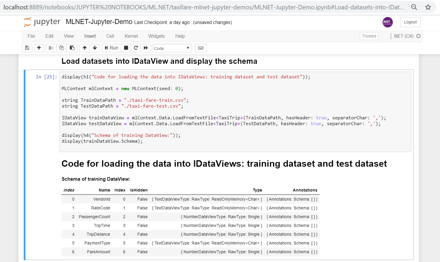
Then, just write the following code and run it so you see the training IDataView schema:
display(h1("Code for loading the data into IDataViews: training dataset and test dataset"));

MLContext mlContext = new MLContext(seed: 0);

string TrainDataPath = "./taxi-fare-train.csv";
string TestDataPath = "./taxi-fare-test.csv";

IDataView trainDataView = mlContext.Data.LoadFromTextFile<TaxiTrip>(TrainDataPath, hasHeader: true, separatorChar: ',');
IDataView testDataView = mlContext.Data.LoadFromTextFile<TaxiTrip>(TestDataPath, hasHeader: true, separatorChar: ',');

display(h4("Schema of training DataView:"));
display(trainDataView.Schema);
Here’s how you see it in Jupyter:
You can also visualize a few rows of the data loaded into any IDataView such as here:
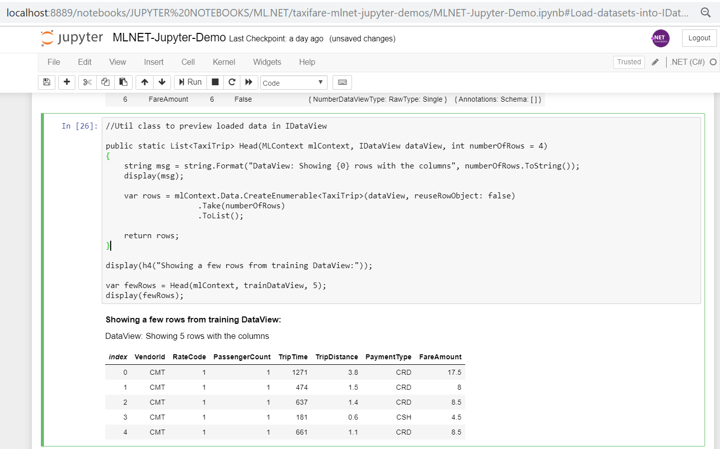
This action is a bit more verbose, but we’re working on another data structure in .NET for exploring data named ‘DataFrame’ very similar to the DataFrame in Pandas in Python which is a lot simpler than when working with the IDataview because the DataFrame is eager instead of lazy loading plus you don’t need to work with typed data classes just for exploring data.
Plotting data with XPlot
XPlot is a popular plotting library in the F# community that you can also use from C#: https://fslab.org/XPlot/
In the initial cell you already installed its Nuget package so now you can simply use it in Jupyter.
Prepare data in arrays
XPlot works with any IEnumerable based type but the most common way is by using arrays, so first of all we’re going to extract some input variables data in a few arrays:
//Extract some data into arrays for plotting:

int numberOfRows = 1000;
float[] fares = trainDataView.GetColumn<float>("FareAmount").Take(numberOfRows).ToArray();
float[] distances = trainDataView.GetColumn<float>("TripDistance").Take(numberOfRows).ToArray();
float[] times = trainDataView.GetColumn<float>("TripTime").Take(numberOfRows).ToArray();
float[] passengerCounts = trainDataView.GetColumn<float>("PassengerCount").Take(numberOfRows).ToArray();
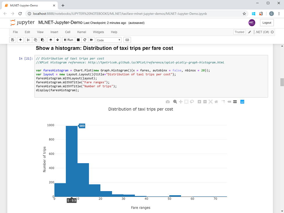
After running that in a Jupyter cell, you can now plot data distributions such as the following histogram where you can see that most of the taxi trips were between $5 and $10.
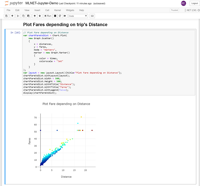
Or more interestingly, you can see how the ‘distance’ input variable impacts the fare/price of the taxi trips, although you can also see that some other variables might be influencing, as well, because when the distance is higher the dots are more sparse probably due to the ‘time’ variable that you can also plot.
You can check the Jupyter notebook file (MLNET-Jupyter-Demo.ipynb) I’m providing and see additional plotting charts I explored.
Create the ML Regression model with ML.NET
Now, let’s get into ML.NET code. We’ll first work on the data transformations then we’ll add the trainer/algorithm and finally we’ll train the model which creates the model itself.
Data transformations in the model pipeline
In order to create a regression model we first need to make some data transformations (convert text to numbers, normalize and concatenate input variables) in our pipeline such as the following:
display(h1("Apply Data Transformations pipeline"));

// STEP 2: Common data process configuration with pipeline data transformations
var dataProcessPipeline = mlContext.Transforms.Categorical.OneHotEncoding(outputColumnName: "VendorIdEncoded",
                                                                          inputColumnName: nameof(TaxiTrip.VendorId))
     .Append(mlContext.Transforms.Categorical.OneHotEncoding(outputColumnName: "RateCodeEncoded",
                                                             inputColumnName: nameof(TaxiTrip.RateCode)))
     .Append(mlContext.Transforms.Categorical.OneHotEncoding(outputColumnName: "PaymentTypeEncoded",
                                                             inputColumnName: nameof(TaxiTrip.PaymentType)))
     .Append(mlContext.Transforms.NormalizeMeanVariance(outputColumnName: nameof(TaxiTrip.PassengerCount)))
     .Append(mlContext.Transforms.NormalizeMeanVariance(outputColumnName: nameof(TaxiTrip.TripTime)))
     .Append(mlContext.Transforms.NormalizeMeanVariance(outputColumnName: nameof(TaxiTrip.TripDistance)))
     .Append(mlContext.Transforms.Concatenate("Features", "VendorIdEncoded", "RateCodeEncoded", "PaymentTypeEncoded",
                                              nameof(TaxiTrip.PassengerCount), nameof(TaxiTrip.TripTime),
                                              nameof(TaxiTrip.TripDistance)));
You should run that code in a new Jupyter cell you create.
If you want to learn more about the data transformations needed for a regression problem, take a look to this tutorial:
https://docs.microsoft.com/en-us/dotnet/machine-learning/tutorials/predict-prices
Add the trainer/algorithm and train the model
In the following code we add the trainer/algorithm SDCA (Stochastic Dual Coordinate Ascent) to the pipeline and then we train the model by calling the fit() method and providing the training dataset:
%%time
var trainer = mlContext.Regression.Trainers.Sdca(labelColumnName: "FareAmount", featureColumnName: "Features");
var trainingPipeline = dataProcessPipeline.Append(trainer);

var trainedModel = trainingPipeline.Fit(trainDataView);
And here’s the execution in Jupyter with just some more ‘displaying info’ lines of code:
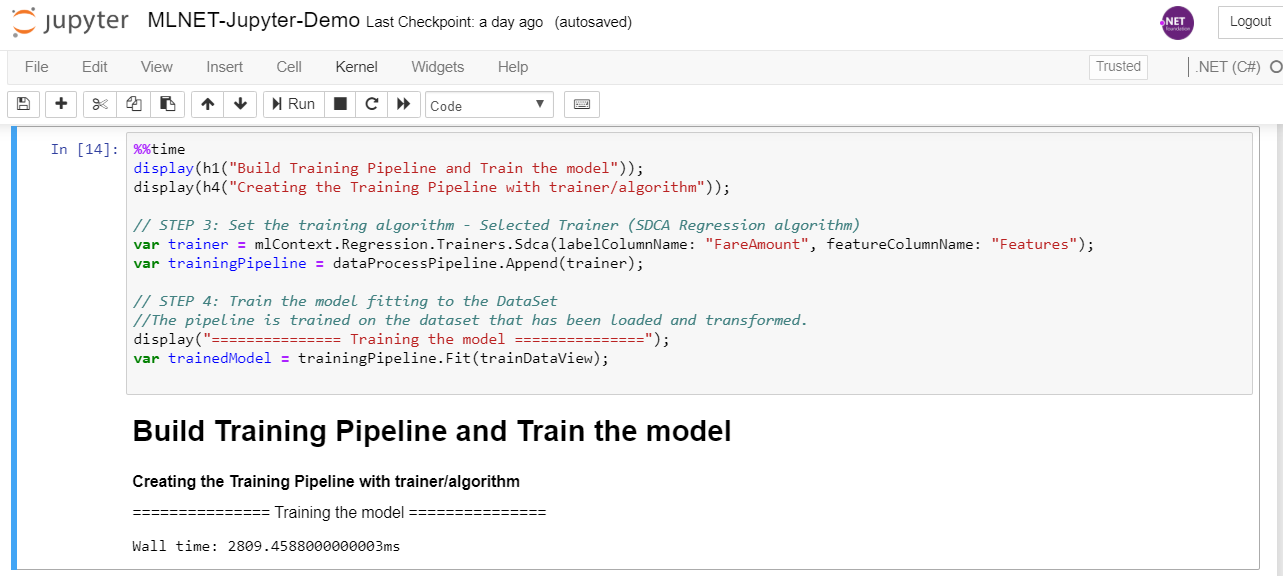
A very interesting thing you can use in C# when running a cell is the ‘%%time’ code which will measure the time it needed to run all the code in that Jupyter cell. This is especially interesting when you know something is going to take its time, like when training an ML model, depending on how much data you have for training. In that case above it tells us it needed almost 3 seconds, but if you have a lot of data it could be minutes or even hours.
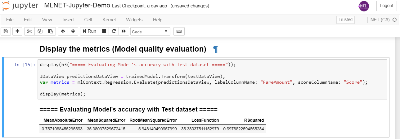
Evaluate the model’s quality: Metrics
Once you have the model another important step is to figure out how good it is by calculating the performance metrics with some predictions that are compared to the actual values from a test-dataset, like in the following code:
IDataView predictionsDataView = trainedModel.Transform(testDataView);
var metrics = mlContext.Regression.Evaluate(predictionsDataView, labelColumnName: "FareAmount", scoreColumnName: "Score");

display(metrics);
Here you can directly see the metrics in the Jupyter notebook in a very neat way by simply calling ‘display(metrics)’ 🙂
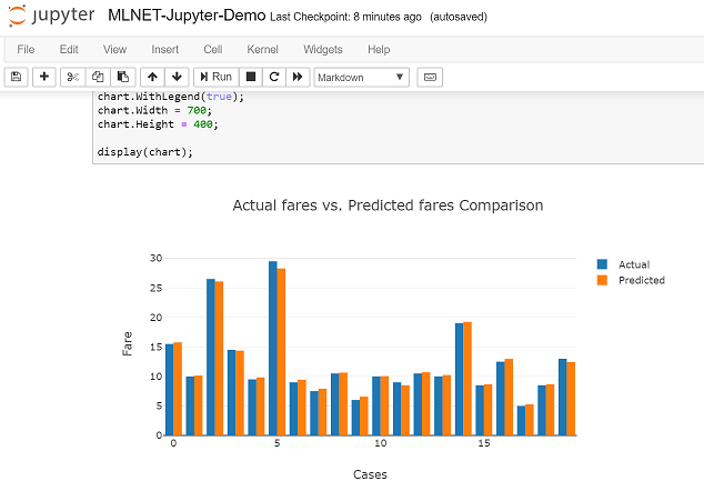
Make predictions in bulk and show a bar diagram comparing predictions vs. actual values
Here’s the code on how to make a few predictions and show in a bar chart a comparison of predictions versus actual values from the test dataset:
// Number of rows to use for Bar chart
int totalNumberForBarChart = 20;

float[] actualFares = predictionsDataView.GetColumn<float>("FareAmount").Take(totalNumberForBarChart).ToArray();
float[] predictionFares = predictionsDataView.GetColumn<float>("Score").Take(totalNumberForBarChart).ToArray();
int[] elements = Enumerable.Range(0, totalNumberForBarChart).ToArray();

// Define group for Actual values
var ActualValuesGroupBarGraph = new Graph.Bar()
{
   x = elements,
   y = actualFares,
   name = "Actual"
};

// Define group for Prediction values
var PredictionValuesGroupBarGraph = new Graph.Bar()
{
   x = elements,
   y = predictionFares,
   name = "Predicted"
};

var chart = Chart.Plot(new[] {ActualValuesGroupBarGraph, PredictionValuesGroupBarGraph});
var layout = new Layout.Layout(){barmode = "group", title="Actual fares vs. Predicted fares Comparison"};
chart.WithLayout(layout);
chart.WithXTitle("Cases");
chart.WithYTitle("Fare");
chart.WithLegend(true);
chart.Width = 700;
chart.Height = 400;

display(chart);
And here’s the bar chart in Jupyter:
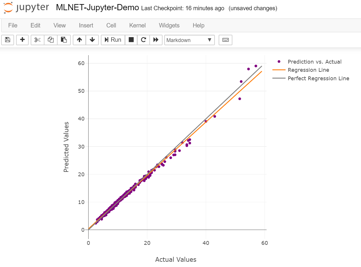
Plotting Predictions vs. Actual values plus the Regression line
Finally, with the following code you can plot the predictions vs. the actual values. If the regression model is working well the dots should be most of them around a straight line which is the regression line. Also, the closer the regression line is to the ‘perfect line’ (prediction is equal to the actual value in the test dataset), the better quality your model has.
Here’s the code:
using XPlot.Plotly;

// Number of rows to use for Plotting the Regression chart
int totalNumber = 500;

float[] actualFares = predictionsDataView.GetColumn<float>("FareAmount").Take(totalNumber).ToArray();
float[] predictionFares = predictionsDataView.GetColumn<float>("Score").Take(totalNumber).ToArray();

// Display the Best Bit Regression Line

// Define scatter plot grapgh (dots)
var ActualVsPredictedGraph = new Graph.Scatter()
{
   x = actualFares,
   y = predictionFares,
   mode = "markers",
   marker = new Graph.Marker() { color = "purple"} //"rgb(142, 124, 195)"
};

// Calculate Regression line
// Get a touple with the two X and two Y values determining the regression line
(double[] xArray, double[] yArray) = CalculateRegressionLine(actualFares, predictionFares, totalNumber);

// Define grapgh for the line
var regressionLine = new Graph.Scatter()
{
   x = xArray,
   y = yArray,
   mode = "lines"
};

// Display the 'Perfect' line, 45 degrees (Predicted values equal to actual values)
var maximumValue = Math.Max(actualFares.Max(), predictionFares.Max());

var perfectLine = new Graph.Scatter()
{
   x = new[] {0, maximumValue},
   y = new[] {0, maximumValue},
   mode = "lines",
   line = new Graph.Line(){color = "grey"}
};

// XPlot CSharp samples: https://fslab.org/XPlot/chart/plotly-line-scatter-plots.html
//Display the chart's figures
var chart = Chart.Plot(new[] {ActualVsPredictedGraph, regressionLine, perfectLine });
chart.WithXTitle("Actual Values");
chart.WithYTitle("Predicted Values");
chart.WithLegend(true);
chart.WithLabels(new[]{"Prediction vs. Actual", "Regression Line", "Perfect Regression Line"});
chart.Width = 700;
chart.Height = 600;

display(chart);
And this is how you’ll see the regression line and plot chart:
Save the ML model as a file
Finally, you can also save the ML.NET model file and see it in the same folder than your Jupyter notebook:
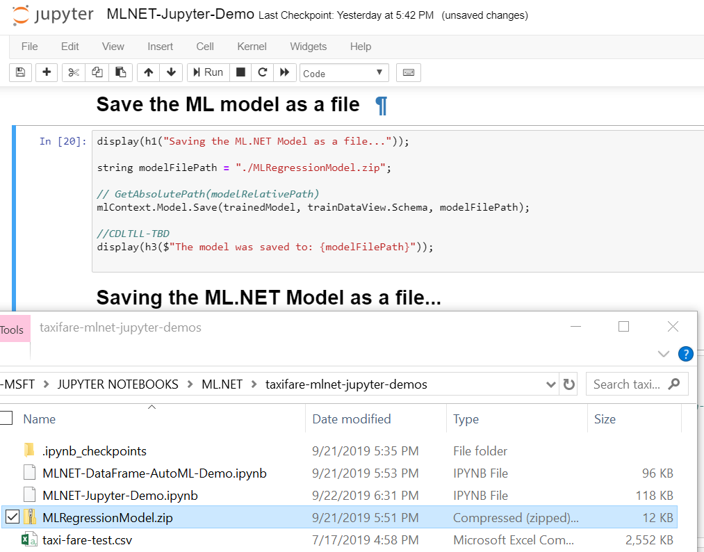
You can the take that .ZIP file (ML.NET model) and deploy it (consume it) in any .NET application like you can see here for making predictions in an Azure Function or an ASP.NET Core app/WebAPI:
- Deploying an ML.NET model into an Azure Function
- Deploying an ML.NET model into an ASP.NET Core app/WebAPI
Conclusions and take aways
Jupyter is a great environment for scenarios such as:
- Data exploration and plotting
- Documenting Machine Learning model experiments and conclusions
- Creating courses based on Jupyter notebooks. Great for many learning scenarios
- Labs or Hands on labs
- Creating quizzes for learning environments
And now with the .NET kernel for Jupyter you can take advantage of it for all those scenarios.
Please, feel free to send us your feedback through this blog post comments or into the following GitHub issues:
dotnet-try feedback: https://github.com/dotnet/try/issues
ML.NET feedback: https://github.com/dotnet/machinelearning/issues
We can’t wait to hear from you about the ideas and assets you can create with Jupyter+ML.NET! 🙂
Happy coding!


0 comments