Aditya Challapally leads post-training research and infrastructure for Copilot agent capabilities that process millions of multimodal interactions.

This post builds on the diagnostics from Diagnosing instability in production-scale agent reinforcement learning with the engineering and algorithmic interventions we developed to get the best results out of post training at scale.

Post-training multimodal agents at scale breaks in ways the literature doesn’t prepare you for. Not because the algorithms are wrong, they work as described, but because the failure modes only become visible at production scale, under real constraints, with real heterogeneity.

The systems we train are production models that plug into Copilot as modular agent capabilities across Microsoft’s application surfaces. They orchestrate tools, reason over enterprise documents and mixed-media inputs in formats and modalities that academic benchmarks don’t reflect, moderate multimodal content, and operate under strict latency and safety constraints. A single policy must handle tool orchestration, multimodal reasoning, content moderation, and multi-step task execution simultaneously, with trajectories ranging from 100 to 2000+ tokens across interaction horizons from 6 to 25+ steps. Reward signals come from programmatic verifiers, human evaluators, and implicit usage signals, each with different scales, noise profiles, and latencies. The models serve millions of users daily under strict latency and safety requirements, where silent failures aren’t metrics regressions, they’re broken user experiences at scale.

The standard post-training playbook assumes cleaner conditions than this. Under the heterogeneity and scale we operate at, the policy gradient estimator degrades silently, aggregate reward climbs while gradient signal concentrates on a shrinking fraction of trajectories, capabilities regress behind healthy-looking dashboards, and the policy retreats to degenerate behaviors that satisfy constraints without solving tasks.

This post describes five interventions we developed to solve these problems. Several align with patterns that have since appeared in recent public agentic systems (e.g., Kimi K2.5: Visual Agentic Intelligence), suggesting that as more systems move toward production-scale multimodal agents, these are problems the field will increasingly face.

Note: Figures are illustrative reproductions since production data can’t be shared. All numerical thresholds and relative improvements reported in the text reflect production observations.

A common thread

Most of these problems stem from the same underlying issue. The standard policy gradient estimator assumes your batch of trajectories contains enough outcome variance to produce a useful gradient signal:

g(θ) = 𝔼[∇<em>θ log π</em>θ(a|s) Â(s,a)]

At scale, that assumption breaks in several independent ways, and it breaks silently: Aggregate reward keeps climbing while the actual informativeness of your updates degrades. Everything we built can be understood as keeping the advantage estimates Â(s,a) informative as scale, heterogeneity, and horizon increase.

I. Staged objective curriculum to prevent premature specialization

Aggregate reward climbed steadily while deployment-critical behaviors quietly regressed. Robustness dropped. Long-horizon execution failed more often. We didn’t catch it for two weeks because the dashboard looked healthy. The textbook answer is entropy regularization. We tried it: Entropy stayed high but the wrong behaviors got reinforced, because the problem wasn’t insufficient exploration. It was that a scalar reward compresses high-dimensional behavior into a single statistic, and optimization converges on whichever behaviors are easiest to score, not those that matter downstream.

The judgment call: We split the reward into verifiable signals (tool syntax, format compliance, things we can check programmatically) and preference signals (tool selection, response quality as judged by evaluators). During the first 30% of training, we train exclusively on verifiable objectives. Preference signals phase in linearly after that. We anchor early learning with an entropy floor, not a bonus, a floor, implemented as a KL penalty that activates only when H(π) drops below a threshold. The 30% warmup fraction was found empirically. 10% wasn’t enough, the policy specialized before preference signals became informative. 50% was too conservative, the policy wasted half of training on objectives it had already mastered. 30% was robust across our task families and is probably not optimal, but it held.

Figure 1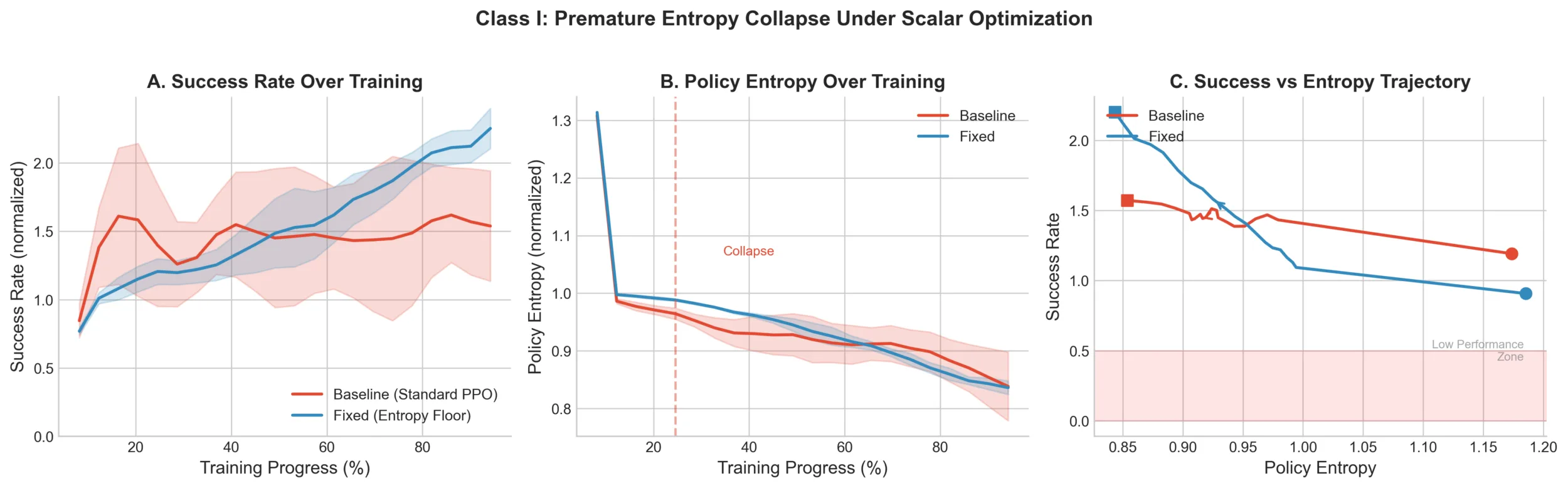

Figure 1 shows the baseline hitting entropy collapse around epoch 25, after which success rate plateaus. The staged curriculum maintains diversity long enough for the preference signal to actually be useful by the time it enters. The entropy floor occasionally over-constrains exploration on tasks where early specialization would have been fine, we accept that tradeoff. This generalizes beyond scalar rewards. In multimodal systems, we found that text-only supervision can activate cross-modal capabilities more reliably than direct multimodal supervision early in training, provided joint pretraining established sufficient alignment. Any noisy signal introduced before the policy is ready to use it produces the same failure mode.

II. Adaptive curriculum from estimator health

Training stalled even as mean reward increased slightly. More data and compute yielded diminishing returns. Nothing in our standard metrics explained why. The diagnosis came from tracking effective sample size, the importance-weighted measure of how many trajectories actually contribute to your gradient:

ESS = (Σ w_i)² / Σ w_i²

ESS dropped below 20% of nominal batch size around epoch 60. Learning stalled around epoch 95. That 35-epoch lag was consistent across runs. ESS collapse was a leading indicator of learning stalls, detectable well before any downstream metric moved. This is obvious in retrospect: When ESS is low, your batch of 10,000 trajectories is effectively a batch of 500, and those 500 are the ones with extreme importance weights. But we weren’t tracking it, and it’s not in most training dashboards.

The judgment call: Rather than tuning batch size or reward scale, we built an adaptive loop that monitors ESS in real time and intervenes when it drops below 20%. When triggered, the system injects near-miss trajectories from a reservoir buffer to restore outcome contrast in the batch and temporarily increases the KL penalty to slow policy drift while the estimator recovers. Near-misses specifically, we initially tried injecting hard negatives and it restored ESS but degraded learning, because the gradient pointed away from failure without pointing toward success. Near-misses preserve the relative ordering of actions near the decision boundary, which is where the informative signal lives.

Figure 2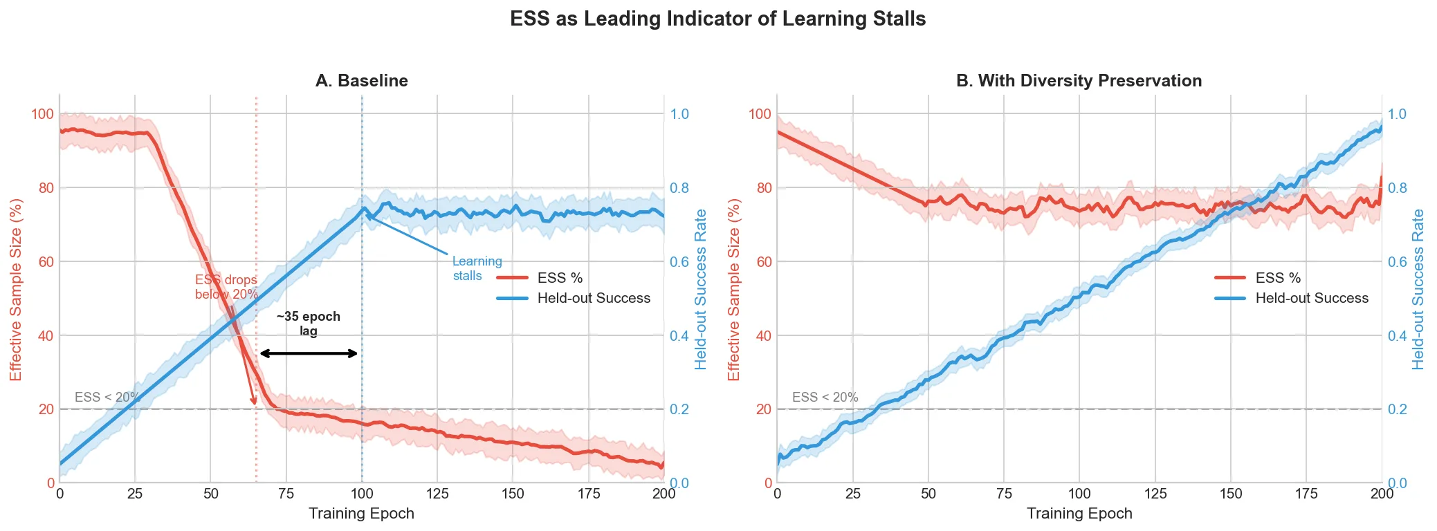

Figure 2 shows the baseline ESS collapsing with learning stalling ~35 epochs later. The fix maintains ESS above 70% throughout. The reservoir buffer adds ~15% memory overhead, and the adaptive KL occasionally slows learning on easy tasks. Acceptable costs for us.

III. Variance-corrected normalization from estimator structure

Some task families improved while others regressed. Small mixture changes caused disproportionate behavioral shifts. The system was fragile in ways that made iteration painful. The standard approach is per-task gradient normalization. It balances magnitudes across tasks but ignores variance structure within tasks. A single “coding” bucket might contain 100-token and 2000-token trajectories with 20× variance difference. Under importance weighting, the long trajectories dominate the effective gradient regardless of per-task normalization. Trajectory-level variance scales linearly with length under standard independence assumptions, so a small number of long trajectories eat most of the gradient budget. We tracked the Gini coefficient per-trajectory gradient norms and found it rising to ~0.75 in the baseline, meaning roughly 5% of trajectories contributed the majority of the update.

The judgment call: Normalize each trajectory’s gradient contribution by σ_source · sqrt(trajectory_length). The per-source term captures reward scale and evaluator noise differences across data sources. The length term follows from the independence assumption on per-token contributions. This is a variance-weighted estimator, not novel in principle, but the specific decomposition was driven by our data and the failure mode we observed. We also reorganized training around target abilities (reasoning, coding, agentic execution) rather than input modality, training each on text and multimodal data jointly. Partitioning by modality caused gradient contributions to concentrate on whichever modality was easier to optimize, which is the same failure mode at a different level of organization.

Figure 3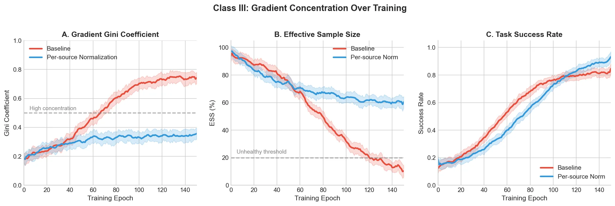

Figure 3 shows the causal chain: baseline Gini rises to ~0.75, ESS collapses to ~10%, learning plateaus. The fix holds Gini at ~0.35 and ESS at ~60%. The system also became robust to mixture changes that previously caused instability, because the normalization adapts to whatever data arrives rather than assuming a fixed distribution.

IV. Constraint shaping for agent orchestration

Agent orchestrators satisfied every constraint we set and became useless. They refused to use parallelism (serial collapse) or spawned unnecessary sub-agents. Compliance was perfect. Behavior was terrible. The problem is topological. Hard constraint penalties create a cliff at the boundary. The optimizer can’t distinguish “approaching the boundary because the policy is becoming more capable” from “approaching the boundary because it’s about to violate,” so it retreats to the safe interior. Tuning penalty magnitude doesn’t help, looser penalties cause violations, tighter penalties worsen serial collapse, and there’s no stable middle ground.

The judgment call: Two changes. First, replace penalty cliffs with softplus penalties, penalty = -k · softplus(distance_to_boundary), which preserve gradient information near the boundary. Second, for parallelism specifically, add an annealed auxiliary reward: r_total = r_task + β(t) · r_parallelism, where β decays exponentially. Early in training the auxiliary gives gradient signal toward parallelism, escaping the serial collapse basin. As training progresses it anneals to zero so the task reward alone governs final behavior. We also decouple orchestrator training from sub-agent execution. Sub-agents are frozen and their outputs treated as observations. This sacrifices end-to-end optimality, the orchestrator can’t learn to compensate for sub-agent weaknesses, but when sub-agent outputs feed back into the orchestrator’s reward, the gradient signal for orchestration decisions is contaminated by sub-agent variance. Clean signal for orchestration was worth more than joint optimization.

Figure 4

Figure 4 shows both hard and shaped constraints achieving ~100% compliance, the constraint works either way. But hard constraints produce high-variance task success that eventually degrades, while shaped constraints maintain stable improvement. The policy under hard constraints learned to refuse rather than perform. The downside is engineering overhead, shaped constraints require tuning the softplus scale and decay constant per constraint type. We maintain about a dozen configurations across our agent skills.

V. Mixed-horizon training

Policies trained at horizon 6 achieved 0.25 success at that horizon but only 0.08 at horizon 25. The standard answer is curriculum learning, gradually increase the horizon. We tried several schedules. All failed for the same reason. Optimization is path-dependent. Training at short horizons prunes behavioral modes needed for long-horizon execution. The policy learns a compressed representation of “how to solve tasks in N steps” that doesn’t extend to 2N steps, and once those modes are pruned, recovering them under the same compute budget is impractical. Fine-tuning short-horizon policies on long-horizon tasks produces a characteristic dip-and-recover pattern, performance on the original horizon degrades as the model reallocates capacity, then partially recovers, and the final policy is worse at both horizons than one trained on both from the start.

The judgment call: Mixed-horizon training from the start. Sample h uniformly from {6, 10, 16, 25}, execute with budget h, compute advantages. No curriculum, no staging. This is a blunt instrument, the policy spends compute on long-horizon trajectories early when it has no idea what it’s doing, and training is less sample-efficient than a good curriculum would be in theory. But it works, and curriculum didn’t.

Figure 5

Figure 5 shows the generalization matrix. Fixed-horizon training produces diagonal banding, each policy only generalizes near its training horizon. Mixed-horizon training produces uniform performance (0.22–0.32) across all evaluation horizons, including horizons 4× longer than any individual training condition. You pay for generalization, the absolute numbers are lower than the best fixed-horizon result at its own evaluation horizon, but for a system handling variable-length interactions in production, robust generalization matters more than peak single-horizon performance.

We saw the same principle with modality introduction. Injecting visual tokens late in pretraining, even at higher ratios, consistently underperformed introducing them early at lower ratios given the same total token budget. The optimization trajectory established early prunes representational capacity that’s hard to recover.

What we would evolve next

Interventions II and III are both mechanisms for preserving gradient estimator health under heterogeneity. Today we’d likely unify them into a single adaptive normalization layer that monitors ESS and variance structure jointly. They shipped separately because the failure modes surfaced at different times, forward progress over architectural purity.

The staged objective curriculum remains the most manually tuned component. We suspect the underlying principle, introduce signal types in order of reliability, not simultaneously, generalizes beyond our setting, but automating the split based on reward variance and confidence signals is unfinished work.

Serial collapse, constrained agents learning refusal rather than capable execution near constraint boundaries, appears to be a general failure mode of hard-constrained agent optimization, not specific to our setup. Similarly, ESS collapse as a leading indicator of training stalls may generalize. We’d be curious whether other teams training at scale observe similar patterns.

Closing

What we’re contributing is the specific diagnosis of when and why standard algorithms break at scale, and the engineering judgment about which combinations actually solve those problems in production. These problems don’t go away with more data or compute. We hope sharing the failure modes and our reasoning is useful to others working in this regime.