Active Learning for Object Detection in Partnership with Conservation Metrics

Olga Liakhovich

Introduction

Using artificial intelligence to monitor the progress of conservation projects is becoming increasingly popular. Potential applications range from preventing poaching of endangered species to monitoring animal populations in remote, hard-to-reach locations. While proven to be extremely effective, computer vision AI projects leverage a large amount of raw image data to train the underlying machine learning models. These images, often captured by drones and/or camera traps, need to be annotated – a manual process of identifying regions of interest and assigning each region a class-label – which can be extremely time-consuming. It’s worth mentioning that some AI solutions may need only hundreds of high-quality labeled images and for others that number could be in the thousands. The need to optimize the labeled dataset preparation step is something that we see very often.

Last year, our team undertook a project in partnership with Conservation Metrics to autonomously monitor the breeding population of an endangered bird species using deep learning. This year, we teamed up with Conservation Metrics again to specifically tackle efficient data labeling for object detection projects.

In this code story, we will introduce the concept of active learning: a semi-supervised machine learning approach in which a learning algorithm is able to query the user to request the desired information needed to label images. This technique allows experts to use trained machine learning models to select the most impactful image sets for annotation. In addition, using active learning, machine learning models are able to propose labels (bounding boxes) that human experts can review, rather than having to do all annotation from scratch.

During our partnership, our CSE team was tasked with creating an end-to-end automated pipeline for active learning that supports deep learning-based object detection models on both Azure Data Science Virtual Machines (with Tensorflow) and the Azure Custom Vision Service.

Challenges and Solution

Labeling image data has traditionally been a tedious task. For example, during our recent collaboration with Conservation Metrics for the bird detection project, it took our team more than 20 hours to manually label just a few hundred images. Wildlife monitoring generally produces thousands of images daily, providing a treasure trove of data accounting for different factors such as weather conditions and camera modes. In order to leverage all this data to build robust machine learning models, it is vital to have an efficient process in place that maximizes the productivity of expensive human experts.

We identified this as an ideal scenario for active learning, which can both decrease the amount of labeled data needed while speeding up the process of experts actually producing the labeled data.

What is Active Learning?

Before delving into the details of the project, let’s first discuss the concept of active learning, as well as the most recent research on this topic. Active learning refers to the subset of machine learning algorithms designed for projects featuring a lot of unlabeled data, in which labeling all that data manually is unfeasible. When using active learning, the algorithm is able to select a smaller subset of the data, and then prompt the user to label it. It’s worth mentioning at this point that the samples aren’t selected at random, but instead there are policies for selecting samples, mainly aimed at minimizing the model’s prediction error.  The best active learning algorithms are able to query the user so as to train with limited labeled data, reduce the effort required for each tag, and create models that can generate explanations along with their predictions.

For this project, we wanted to find an active learning approach that would be capable of reducing the amount of labeled data needed. There are three general categories of this type of algorithm:

1. Membership query synthesis: the algorithm generates its own examples which it uses to prompt the user to label images, and focuses on creating examples that it believes will best improve its performance.
2. Stream-based selective sampling:  the algorithm is given a stream of data, and has to determine whether or not it wants to label each element in the stream. The main focus is on predicting the importance of each individual element in the stream.
3. Pool-based active learning: the algorithm is given a large pool of unlabeled data and can select any subsection of that pool to be labeled. The algorithm will compare all of the images in the pool to find the most useful ones to label.

Considering the fact that Conservation Metrics had access to a large pool of data from previous projects which they wanted to use to train the model, plus new images which are constantly being added, our team chose to focus on the pool-based active learning technique. We chose uncertainty sampling to select samples, as these images are the “hardest” to process, and using a challenging training set was more likely to cause the model to make more accurate predictions.

The solution

Creating an active learning pipeline

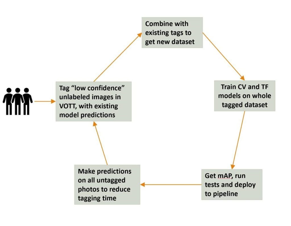
Figure 1: The active learning workflow we designed (some terms like VOTT and mAP are explained in the body.

Our pipeline for Active Learning operates on the same principle as the workflow depicted in Figure 1, but slightly simplified as shown in Figure 2.  Predicted bounding boxes are displayed in the Visual Object Tagging Tool (VOTT) where a human verifier corrects the boxes before uploading the dataset for next iteration of training.

Figure 2: A simplified active learning workflow.

Using our system, an annotator labeled a base set of images without predictions, before uploading them to an Azure Blob Storage account holding all the tags. They then trained the first iteration of the model using either an Azure Data Science Virtual Machine (with Tensorflow Object Detection) or the Azure Custom Vision Service. After this, the trained object detection model produced predictions for all of the unlabeled images. Finally, the images with the most uncertainty (lowest confidence in the predicted classes) were prioritized for manual review by a human annotator and the cycle repeated.

A key element to driving efficiency is that predictions produced by the current version of the model are displayed on the images during the next round of tagging. This allowed the human annotator to simply focus on reviewing labels (bounding boxes) and making any corrections which were necessary. As a further step to speed things up, our pipeline was designed to support the work of multiple taggers working at any one time.

Using active learning for bird detection

During this second partnership with Conservation Metrics, we used active learning labeling to improve the accuracy of the bird detection model described in our earlier blog post. We used active learning to increase the original kittiwakes training set by 20%  and then measured the impact in terms of mean average precision (mAP) performance on the test set.

Figure 3 below demonstrates how much easier it is for human teams to efficiently label images which have been pre-tagged by a machine learning model. White bounding boxes indicate high confidence regions which need to be reviewed by an expert, while red boxes indicate regions that likely require adjustment:

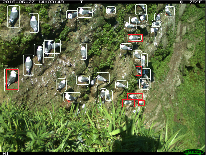
Figure 3: An image pre-labeled by a partially trained model. White rectangles indicate areas of high confidence; red triangles are regions of low confidence and require human adjustment.

Model performance during training is shown on Figures 4 and 5 below. The X-axis shows the number of training iterations, while the Y-axis shows the validation set mAP (mean Average Precision).

Figure 4: Validation set mAP using the original training set (400 images) reaches 91.53%:

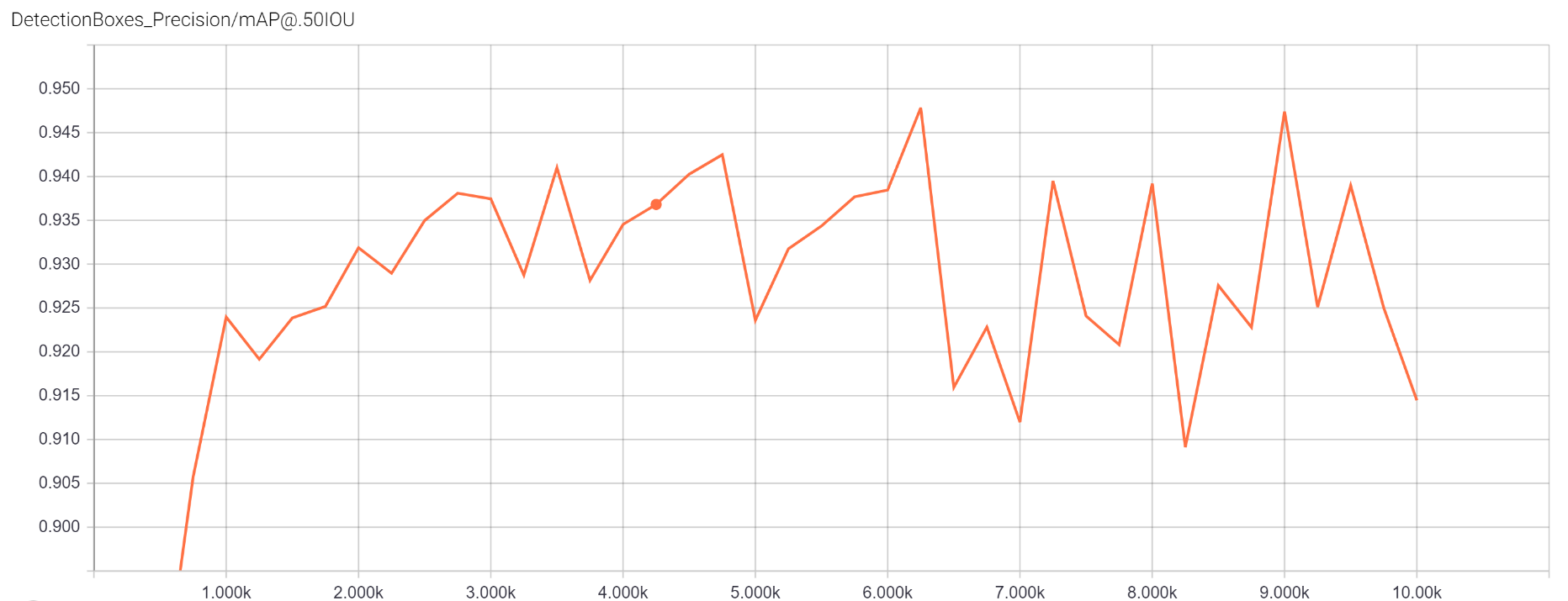
Figure 5 Validation set mAP using a training set boosted by active learning (now 500 images) reaches 94.78%

These results show a noticeable improvement in performance, even after less than 45 minutes of human effort tagging images. Considering that the original data set took almost 20 hours to tag, this gave our team confidence that the active learning algorithm was accurately predicting which images needed to be reviewed by a human tagger, increasing efficiency per labeled image overall and reducing the time needed to review images.

Scripts for the DSVM + Tensorflow object detection pipeline

Here we outline the key scripts we developed   (see project GitHub repository) to run the pipeline on the Data Science Virtual Machine and Tensorflow Object Detection. You can also find a video walk-through showing how to run the entire pipeline below:

Let’s go over each step of the tagging process: 

1. Initializing the pipeline.

We decided that the workflow should start with images being downloaded to the tagging machine and that the state of the pipeline  — in this case, the list of images to be labeled — should be stored in persistent storage. To keep the workflow setup lightweight we opted against provisioning databases and instead used Azure Blob Storage to track the state of the pipeline. We then used the initialization script active_learning_initialize.sh to save a list of images to be tagged in CSV on the blob — totag.csv.

2.  Choosing images for labeling.

We needed to move a set of images from Azure Blob Storage to the client machine so that the human expert could assign labels. This was done using download_vott_json.py. We implemented customizable logic on how images for tagging are selected: the default option is to pick the k images with the lowest object detection confidence, where k is a user-specified number. In case there are multiple objects in the image, we use the lowest confidence of a predicted bounding box as the confidence value for the whole image.  Another option is using the average, or weighted average, of confidence values.

After this step, the state of the pipeline was saved in a CSV file tagging.csv  — using the list of images reviewed by each human expert. This would allow multiple people to participate in image labeling without having to cross-verify tags.

Initially, users had to draw all bounding boxes from scratch, but after doing a few cycles of active learning, users were able to focus more on verifying and adjusting bounding boxes predicted by the model. The script download_vott_json.py converts a model’s predictions (if they are present) to bounding boxes to be displayed by VOTT. We implemented a custom configuration setting that limits the number of “bounding boxes per pixel”. We found that limit very useful when working on Conservation Metrics’ scenario involving detection of multiple small kittiwakes in an image, as it prevented multiple low-accuracy predictions crowding up the user’s screen and overall made labeling easier for our experts.

3.  Committing labeled data.

The next step addressed the stage when the human experts had finished labeling the images in VOTT (upload_vott_json.py). Bounding box information assigned to each image was converted by the script from the VOTT format (json file) to a generic CSV format — tagged.csv.

Figure 6 below demonstrates the transformation:

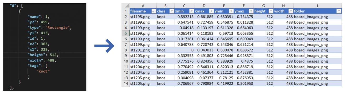
Figure 6: Bounding Box information converted from JSON to CSV.

This data was then used as input to train the object detection model.

4.   Training the model to create predictions.

Our team then combined the next phase of the workflow in the bash script active_learning_train.sh.  This trains the new model based on the latest tagged data, creates new predictions on all of the unlabeled images (including a confidence metric that would determine the priority with which images are sent to taggers) and calculates the model’s performance using either COCO or PASCAL 2007/2012 evaluation techniques.

Below you will find a summary of the most critical parts of active_learning_train.sh:

a) Update_blob_folder.py  and convert_tf_record.py

The first script compares the current images directory on the tagging machine to the blob folder where all the images are stored, and then downloads any required images that are not on the tagging machine. The second script downloads the latest tags from blob storage and bundles them with the downloaded images to create a tf_record (the format used by Tensorflow for ingesting data) which can subsequently be used for training and validation.

b) Train.py and export_inference_graph.py

These scripts are part of the Tensorflow object detection library. They were used to train the object detection model using the downloaded pre-trained model, pipeline config file, and the aforementioned tf_record files before exporting its frozen inference graph for prediction purposes.

c) Create_predictions.py

This script uses the model to make predictions on all images, both labeled and unlabeled, before storing the results in two separate files. When making predictions on unlabeled images, it also uses the user-modifiable calculate_confidence function to generate a confidence score which is then used to determine which images to tag. The predictions for unlabeled items are used to pre-populate bounding boxes in VOTT when a user starts a session to tag images, while the labeled predictions are used for measuring model performance.

d) Map_validation.py

This script calculates the standard object detection metrics, using the ground truth tags provided by the human expert as well as the predictions made by the model. This script supports the COCO mAP metric as well as the PASCAL 2007 and 2012 metrics. The results are stored along with the model inference graph so that a user can easily decide which model performs best to use for deployment.

Enabling active learning with an Azure Custom Vision-based pipeline

As our team was designing the active learning pipeline, we considered using various different options for the machine learning “backend” infrastructure where the object detection model would be (re)trained and where drafts of new tags would be created. The new Azure Custom Vision Service provides object detection functionality as well as the ability to retrain models, and as such was a suitable alternative to using a Data Science VM-based approach in scenarios in which detailed model or training customization was not necessary.

Below is a walk-through of the code we developed to enable active learning with Azure Custom Vision Service:

1. initialize_vott_pull.py

This python script downloads all images to the tagging machine and adds references to a CSV file called totag.csv. All tagging machines use this file to source data.

2. download_vott_json.py

This script looks at totag.csv files and picks the k images with the lowest levels of accuracy, where k is a user-specified number. It then moves the filenames of these images to the file tagging.csv, so they would not be tagged by any future annotators. If there were any predictions logged on these images, the script will convert these predictions into VOTT tags, limited to j tags per pixel, where j is a user-specified number. This prevents multiple low-accuracy predictions crowding the user’s screen, which could complicate the process.

3. upload_vott_json.py

After a user has finished tagging in VOTT, this script converts their tags into a CSV format, adding them to tagged.csv. These tags can then be used to train the model.

4. cv_train.py

This final script updates the Custom Vision Sevice project to ensure that any tagged images added to the blob storage are updated on the user’s custom vision project. It then trains the custom vision model using the newest batch of images and uses the latest iteration to make predictions for all the remaining unlabeled images. Finally, it runs the same mAP validation process used for the DSVM + Tensorflow approach to measure performance.

Writing customized image selection policy

Experts have domain knowledge which will influence their decision. For example, if a postal company was using object detection to detect recipient mailing addresses on envelopes, domain experts know that each envelope should have exactly one recipient mailing address.  In such case  they would be able to assign any examples returned with zero addresses, or more than two detected address regions, a low confidence score.

We implemented the image selection policy for the active learning pipeline in the script create_predictions.py. In order to customization the calculation of the confidence score that is used to select images for review, a developer would change the logic in the calculate_confidence function:

def calculate_confidence(predictions):
   if len(predictions)!=1:
      return 0
   return np.mean([float(prediction[0]) for prediction in predictions])

During our engagement with Conservation Metrics, our team observed that users would often use similar domain knowledge to limit how many tags that they wanted to verify and display in VOTT, since it was time-consuming to remove multiple tags on the same object until left with just one. To deal with this, our config file defined an optional variable called max_tags_per_pixel, which could be used with download_vott_json.py to limit the number of tags encompassing single point on an image.

If config setting max_tags_per_pixel = 1  then only predictions with the highest confidence within a neighborhood will be reviewed by a human expert. When we used this setting with the bird detection scenario, we observed that there were often occasions when 2-3 birds were nesting next to each other — thus we decided that it would be more appropriate to set max_tags_per_pixel  as 2 for this specific project.

# This initializes an array of all zeros, where num_tags[I,j] represents the number of tags in the pixel at row I and column j
num_tags = np.zeros((int(predictions[0][HEIGHT_LOCATION]),int(predictions[0][WIDTH_LOCATION])), dtype=int)
# Before adding a tag, this code checks whether or not any portion of the region that tag covers already has max_tags_per_pixel tags on it. If so, it does not add the tag as that would exceed max_tags_per_pixel.
if np.amax(num_tags[y_1:y_2, x_1:x_2])<max_tags_per_pixel:
   # <Code to add tag>
   # It then increments the area of the tag by one to indicate another tag has been added in those pixels
   num_tags[y_1:y_2, x_1:x_2]+=1

Another image selection technique that we explored was leveraging the intersection over the minimum area, instead of using the standard IoU (intersection over union) for non-maximum suppression (NMS).  The standard NMS method greedily merges the higher scoring proposals with lower scoring ones when the IoU between them is large enough (e.g. IoU >0.5).  We observed issues with this standard approach when working on the birds detection scenario — often 2 or 3 different objects were overlapping with one object being in the foreground (e.g. two birds sitting on the same nest). In this case predicted bounding boxes should overlap and should not be merged, even though the IoU is less than NMS threshold.

An example snippet of code for this scenario can be found below:

cur_x_min = det_x_min[cur_indices_to_keep]

cur_x_max = det_x_max[cur_indices_to_keep]

cur_y_min = det_y_min[cur_indices_to_keep]

cur_y_max = det_y_max[cur_indices_to_keep]

intersect_widths = (np.minimum(cur_x_max[0], cur_x_max[1:]) - np.maximum(cur_x_min[0], cur_x_min[1:])).clip(min=0)

intersect_heights = (np.minimum(cur_y_max[0], cur_y_max[1:]) - np.maximum(cur_y_min[0], cur_y_min[1:])).clip(min=0)

intersect_areas = intersect_widths*intersect_heights

# Inclusion exclusion principle!

minimum_areas = np.minimum((cur_x_max[0]-cur_x_min[0])*(cur_y_max[0]-cur_y_min[0]), (cur_x_max[1:]-cur_x_min[1:])*(cur_y_max[1:]-cur_y_min[1:]))
# Just in case a ground truth has zero area
iomin = np.divide(intersect_areas, minimum_areas, out=minimum_areas, where=minimum_areas!=0)

In the code snippet above, the iomin variable contains all the intersection over minimum area values and could be used to filter tags as the user desired.

Future Recommendations and Research

Active learning is an area of ongoing research. In this section, we provide pointers to relevant studies  and external use cases which may be of interest to anyone considering a similar project:

• Using active learning to classify radiology reports, achieving an F-Score of 95% using <8% of the available training data  (see “Supervised machine learning and active learning in the classification of radiology reports” by Nguyen et al., 2014),
• Creating classifiers that can provide explanations for each classification (see “Training Classifiers with Natural Language Explanations” by Hancock et al, 2018)
• Training an object detection model using humans only for verification, not to draw new object bounding boxes (see “We don’t need no bounding-boxes: Training object class detectors using only human verification” by  Papadopoulos et al., 2016).

In our work with Conservation Metrics, we used an uncertainty sample as the primary technique for image selection to define which images needed to be reviewed by human experts. However, it is important to note that using uncertainty sampling is not a perfect solution and can lead to some problems. For example, the active learning pipeline will fail to recognize cases where the model has high confidence but has predicted incorrectly.

One way to address this problem would be training an autoencoder on images in a training set and then using the autoencoder to reconstruct images from an unseen data set. A high reconstruction loss is an indication that the image differs from the training images, and hence would be more suitable for manual labeling. For further information on this technique look at “Active learning based autoencoder for hyperspectral imagery classification” by Sun et al., 2016. The easier (and potentially much cheaper to implement) option to mitigate pitfalls with uncertainty sampling would be to stochastically select a few high-confidence samples  and ask human experts to review those as well.

Another notable study is “Localization-Aware Active Learning for Object Detection” by Kao et al., 2018. They discuss different approaches to choose selection metrics in order to optimize which images to pick for human review.

During this project we worked with the assumption that trusted human labelers with a sufficient amount of domain expertise  were reviewing the images. Some projects might benefit from having multiple human experts assign labels to the same image with subsequent voting to assign the label.

Conclusion

During this second partnership with Conservation Metrics, we successfully applied active learning methods for Computer Vision in the context of a wildlife monitoring project. We would like to highlight the following takeaways from this project:

• Labeling images that have already been preprocessed by a machine learning model was considerably faster than doing so manually from scratch. When using this approach, human experts (biologists) needed only to draw bounding boxes around the few remaining kittiwakes that were missed by the AI.
• Model performance (mAP) increased significantly when using the enhanced training sets, translating directly into more accurate detection of birds captured images.

We were impressed by the speed at which biologists from Conservation Metrics completed data preparation and image labeling tasks for other wildlife monitoring datasets (e.g. identification of petrels’ eggs thieves). Using the active learning pipeline, it took the Conservation Metrics team just a few days to label thousands of photos taken by camera traps. Having labeled data available allowed us to better train our AI solution. Specifically in training a baseline machine learning model and in the evaluation of the initial results.

This collaboration demonstrated that developing an AI solution is an iterative and continuous process: from data preparation to training and evaluation a model and back to enhancing training data. Our future plans include using this pipeline for a variety of computer vision related projects, including video processing and redaction, electronic document processing, and quality assurance at factories.

We encourage any teams working on object detection projects requiring manual labeling of a large number of images to reference our GitHub repository which can be found here.

Further References

• Documentation about Azure Data Science Virtual Machine.
• Tensorflow Object Detection details.
• Documentation about Azure Custom Vision Service.
• Project GitHub repository.

Olga Liakhovich

Follow