Classifying Leaks Using Cognitive Toolkit

Michael Lanzetta

Background

We recently worked with our partner Sierra Systems on behalf of Pure Technologies, a company that searches for leaks and damage to oil and water pipelines through audio analysis. They accomplish this task by rolling a sensor ball through a pipeline and capturing high-resolution audio data. Previously, they had been using existing audio-based techniques to locate possible anomalies by a tedious, manual classification process. Technicians visually scanned and listened to long segments of the recordings to identify irregularities to determine if various sounds were indeed leaks and, if so, their severity. Since this method took days to analyze the lengthy recordings, we were asked to work with Sierra to design a solution which would reduce classification time.

The Problem

Could we come up with a solution for classifying these anomalies more quickly and with greater accuracy?

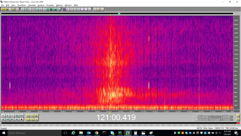
We noticed that if we converted the audio data to a visual representation of its frequency domain and zoomed in, most of the leaks stood right out. We wondered if we could use that observation with the latest in visual classification technology, Convolutional Neural Networks (CNNs), to identify leaks from non-leaks and perhaps even perform finer-grained classification (such as severity or type).

Audio Sampling

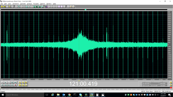
The audio is sampled at 44KHz with 16-bit accuracy in WAV format. These high fidelity recordings capture a variety of different sounds as the sensor ball rolls through the pipe like leaks, gas pockets, obstructions, bends in the pipe and even external noises such as a river or stream crossing. The location of the ball in the pipe is critical to determine the cause of the audio anomaly; as such, the ball not only captures audio but also emits noises at regular intervals to external sensors so that its location can be precisely calculated at any point in time. This extra information helps to eliminate false positives and provide a confidence factor when classifying audio anomalies as leaks. While this additional data was out of scope for the hackfest, it could be added to the project in the future.

Example Leak Audio

The Solution

Building the images

We used basic audio methods to identify likely stretches of the audio file as leaks, which allows us to ignore most of the empty stretches. For the suspect ranges, we walk through the audio file chunk by chunk and convert data into images by performing a Fast Fourier Transform (hereafter FFT). We then annotate the resulting data with its time offset, sample offset and statistics (min/max/mean). Next, we convert these slices of frequency data to images by aggregating over both the frequency and time ranges using the mean values.

Initially, we used a stride of one second and aggregated data to 128×128 images. We eventually used a longer stride and 256×256 images, which produced sharper results. Additionally, we noticed that for more subtle leaks we could use dynamic contrast adjustment to bump up/down intensities within given slices based on their min/max values.

We use Numpy and Scipy heavily – to read the WAV files and to then process them using FFT:

import numpy as np
import scipy.io.wavfile
import math

sampling_rate, data = scipy.io.wavfile.read(wave_file)
# ... code elided for brevity ...
for sec in secs_range:
    start_ix = int(sec * sampling_rate)
    end_ix = int((sec + num_secs_per_img) * sampling_rate)
    cur_img = []
    for ix in range(start_ix, end_ix, int(window_size / 2)):
        cur_fft_mag = np.abs(np.fft.rfft(window * data[ix:ix + window_size]))
        cur_img.append(cur_fft_mag)

We can then take a set of these vectors and save them as an image, in our case using matplotlib’s color-maps to allow us to produce color values (although we’ve found that greyscale does just as well in the production solution):

from scipy.misc import imsave, imresize
from sklearn.preprocessing import MinMaxScaler
from matplotlib import cm
def cvt_to_colormap(data, cmap):
    minv, maxv = np.min(data), np.max(data)
    return [cmap((v - minv) / (maxv-minv)) for v in data]

def arr_to_img(cur_img):
    scaled_data =  MinMaxScaler((0,1000)).fit_transform(np.array(cur_img))
    cur_img_arr = cvt_to_colormap(scaled_data, cm.gist_ncar)
    imsave('./img{}.png'.format(sec), \
      np.rot90(imresize(cur_img_arr, (width, height), 'bicubic')), format='png')

Choosing a Network

We first thought about the potential of taking the sequential amplitude data and using a Recurrent Neural Network. Since we based our initial insight on visualization, however, we chose to approach the problem via Convolutional Neural Networks instead. (It didn’t hurt that CNNs train faster, and we were working on the problem in a weeklong hackfest.)

Our goal for the hackfest was to validate the potential of the approach, not to build the most accurate model, so we chose VGG9 (from the Visual Geometry Group) as our base. This choice had the fringe benefit of being the example in the CNTK Layers tutorial, so we could assume that it worked (we were working on early CNTK 2 Beta code at the time). Since the hackfest, we’ve been evaluating other networks and the potential for ensembling. In our published code, we use ResNet18 and Transfer Learning to build our model.

We created a VGG9 model with Batch Normalization within CNTK using CNTK’s Python binding:

def create_vgg9_model(inputs, out_dims):
  with default_options(activation=relu):
    model = Sequential([
             Convolution((3, 3), 32, init=glorot_uniform(), pad=False),
             BatchNormalization(map_rank=1),
             Convolution((3, 3), 32, init=glorot_uniform(), pad=False),
             BatchNormalization(map_rank=1),
             MaxPooling((3, 3), strides=(2, 2)),
             LayerStack(2, lambda i: [
               Convolution((3, 3), [32, 64, 128][i+1], init=glorot_uniform(), pad=True),
               BatchNormalization(map_rank=1),
               Convolution((3, 3), [32, 64, 128][i+1], init=glorot_uniform(), pad=True),
               BatchNormalization(map_rank=1),
               MaxPooling((3, 3), strides=(2, 2))
             ]),
             LayerStack(1, lambda: [
               Dense(128, init=glorot_uniform()),
               BatchNormalization(map_rank=1)
             ]),
             Dense(out_dims, init=glorot_uniform(), activation=None)
           ])
  return model(inputs)

Training the Network

For our initial training, we took our incoming audio data and processed it as outlined above, producing a set of images. These were labeled based on the location and time of known leaks, including some extra records around the leak to provide a reasonable set of positive examples (leaks are relatively uncommon, thankfully). We further expanded upon the positive results by using some standard data augmentation methods (cropping, shearing, mild rotation) to produce a final set of images. Using CNTK’s ImageReader, we divided the resulting image library into a training and validation set, and trained our model, while keeping a test set holdout for final performance judgment.

We create the train/validation reader from the set of images using CNTK’s MinibatchSource and ImageDeserializer:

import cntk.io.transforms as xforms
def create_reader(map_file, train):
  """
  Define the reader for both training and evaluation action.
  """
  # transformation pipeline for the features has jitter/crop only when training
  transforms = []
  if train:
    transforms += [ xforms.crop(crop_type='randomside', side_ratio=0.8, jitter_type='uniratio') ]
  transforms += [ xforms.scale(width=image_width, height=image_height, \
                                            channels=num_channels, interpolations='linear') ]
  deserializer = ImageDeserializer(map_file, StreamDefs(
                                   features=StreamDef(field='image', transforms=transforms),
                                   labels=StreamDef(field='label', shape=num_classes)
                                  ))
  return MinibatchSource(deserializer)

Building the Pipeline

Our goal for the system is to provide a solution for the partner to score incoming audio files on a regular basis but retrain and recalibrate their model less frequently. Also, we want them to be confident that their model is providing the right results, and enable them to provide feedback (in the form of more labeled data or even refined labels) as time goes on.

We adapted our image generation pipeline to generate “ribbons” of images for large swatches of the audio data, which lets the technician quickly page through the audio file visually and key in on important areas. They can go back through previously generated data and potentially tag it with labels once they’ve validated the results in the field. They can also add additional labels so that in the future we can train higher fidelity models that detect other sub-classes of leaks. Ideally, these models will be able to start identifying pre-leak conditions by tagging previous data from the same location once a leak has surfaced.

Opportunities For Reuse

Developers who are dealing with audio data and would like to classify snippets could make use of the knowledge from this code story. Our approach applies more generally, too, as a way for people to think about data in alternate domains. If you can find a way to convert other types of data into the visual domain, you can then use standard CNN methods to attempt classification.

Please report back to us if you decide to use these ideas in other domains to do something interesting!

Michael Lanzetta ML Manufacturing Lead, Applied ML, CSE

Follow