Considerations of Data Partitioning on Spark during Data Loading on Clustered Columnstore Index

Sumit

Authors: Sumit Sarabhai and Ravinder Singh

Reviewers: Arvind Shyamsundar, Denzil Ribeiro, Davide Mauri, Mohammad Kabiruddin, Mukesh Kumar, and Narendra Angane

INTRODUCTION

Bulk load methods on SQL Server are by default serial, which means for example, one BULK INSERT statement would spawn only one thread to insert the data into a table. However, for concurrent loads you may insert into the same table using multiple BULK INSERT statements, provided there are multiple files to be read.

Consider a scenario where the requirements are:

• Load data from a single file of a large size (say, more than 20 GB)
• Splitting a file isn’t an option as it will be an extra step in the overall bulk load operation.
• Every incoming data file is of different size, which makes it difficult to identify the number of chunks (to split the file into) and dynamically define BULK INSERT statements to execute for each chunk.
• The size of file(s) to be loaded spans through several GBs (say more than 20 GB and above), each containing millions of records.

In such scenarios utilizing Apache Spark engine is one of the popular methods of loading bulk data to SQL tables concurrently.

In this article, we have used Azure Databricks spark engine to insert data into SQL Server in parallel stream (multiple threads loading data into a table) using a single input file. The destination could be a Heap, Clustered Index* or Clustered Columnstore Index. This article is to showcase how to take advantage of a highly distributed framework provided by spark engine by carefully partitioning the data before loading into a Clustered Columnstore Index of a relational database like SQL Server or Azure SQL Database.

The most interesting observation shared in this article is to exhibit how the Clustered Columnstore Index row group quality is degraded when default spark configurations are used, and how the quality can be improved by efficient use of spark partitioning. Essentially, improving row group quality is an important factor for determining query performance.

*Note: There could be some serious implications of parallel inserting data into Clustered Index as mentioned in Guidelines for Optimizing Bulk Import and The Data Loading Performance Guide These guidelines and explanations are still valid for the latest versions of SQL Server.

Environment Setup

Data Set:

• Custom curated data set – for one table only. One CSV file of 27 GB, 110 M records with 36 columns. The input data set have one file with columns of type int, nvarchar, datetime etc.

Database:

• Azure SQL Database – Business Critical, Gen5 80vCores

ELT Platform:

• Azure Databricks – 6.6 (includes Apache Spark 2.4.5, Scala 2.11)
• Standard_DS3_v2 14.0 GB Memory, 4 Cores, 0.75 DBU (8 Worker Nodes Max)

Storage:

• Azure Data Lake Storage Gen2

Pre-requisite: Before going further through this article spend some time to understand Overview of Loading Data into Columnstore Indexes here: Data Loading performance considerations with Clustered Columnstore indexes

In this test, the data was loaded from a CSV file located on Azure Data Lake Storage Gen 2. The CSV file size is 27 GB having 110 M records with 36 columns. This is a custom data set with random data.

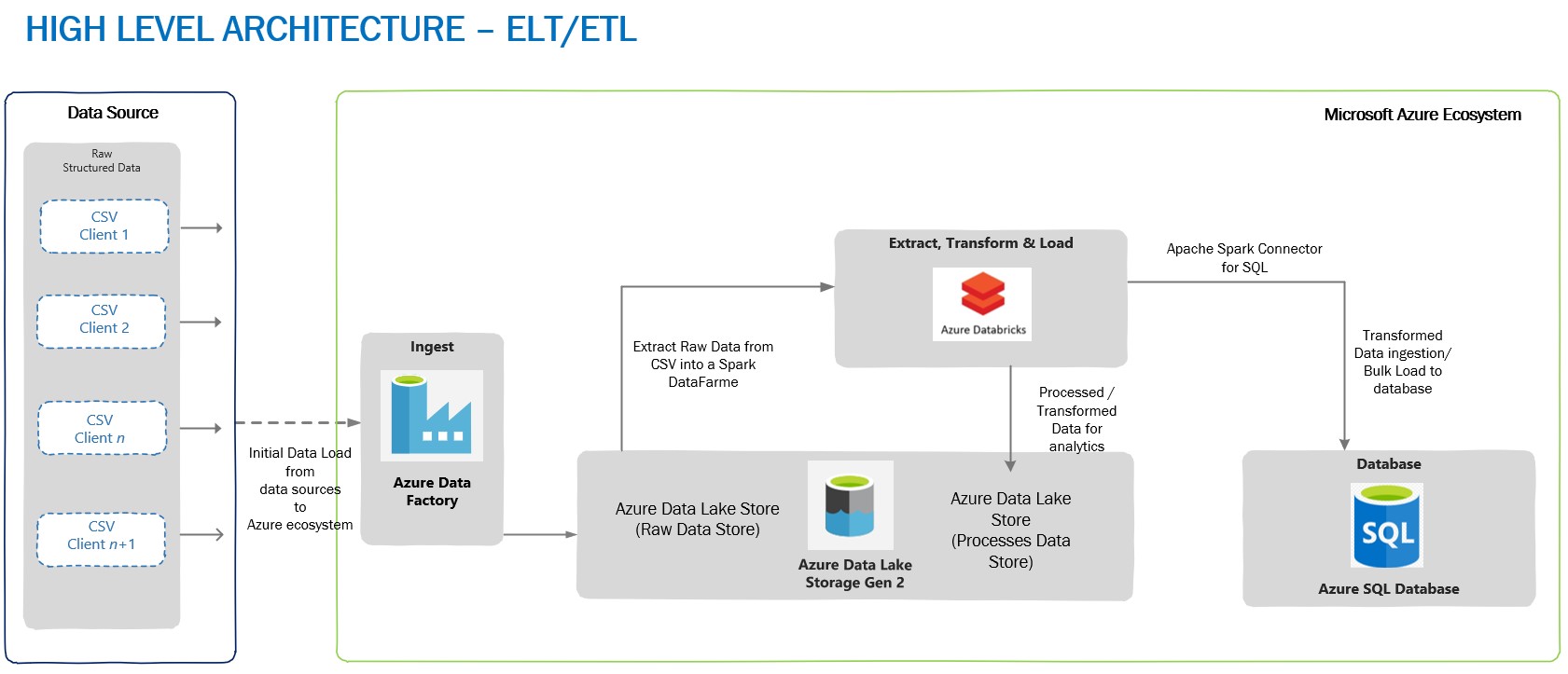
A typical high-level architecture of Bulk ingestion or ingestion post-transformation (ELT\ETL) would look similar to the one given below:

Loading Through BULK INSERTS

In the first test, a single BULK INSERT was used to load data into Azure SQL Database table with Clustered Columnstore Index and no surprises here, it took more than 30 minutes to complete, depending on the BATCHSIZE used. Remember, BULK INSERT is a single threaded operation and hence one single stream would read and write it to the table, thus reducing load throughput.

Loading Through Azure Databricks

To achieve maximum concurrency and high throughput for writing to SQL table and reading a file from ADLS (Azure Data Lake Storage) Gen 2, Azure Databricks was chosen as a choice of platform, although we have other options to choose from, viz. Azure Data Factory or another spark engine-based platform.

The advantage of using Azure Databricks for data loading is that Spark engine reads the input file in parallel through dedicated Spark APIs. These APIs would use a definite number of partitions which are mapped to one of more input data files, and the mapping is done either on a part of the file or entire file. The data is read into a Spark DataFrame or, DataSet or RDD (Resilient Distributed Dataset). In this case data was loaded into a DataFrame which was followed by a transformation (setting the schema of a DataFrame to match the destination table) and then the data is ready to be written to SQL table.

To write data from DataFrame into a SQL table, Microsoft’s Apache Spark SQL Connector must be used. This is a high-performance connector that enables you to use transactional data in big data analytics and persists results for ad-hoc queries or reporting. The connector allows you to use any SQL database, on-premises or in the cloud, as an input data source or output data sink for Spark jobs.

Bonus: A ready to use Git Hub repo can be directly referred for fast data loading with some great samples: Fast Data Loading in Azure SQL DB using Azure Databricks

Note that the destination table has a Clustered Columnstore index to achieve high load throughput, however, you can also load data into a Heap which will also give good load performance. For the relevance of this article, we’ll talk only about loading into a Clustered Columnstore Index. We used different BATCHSIZE values for loading data into a Clustered Columnstore Index – please refer this document to know the impact of BATCHSIZE during bulk loading into Clustered Columnstore Index.

Below are the test runs of data loading on Clustered Columnstore Index with BATCHSIZE 102,400 and 1,048,576:

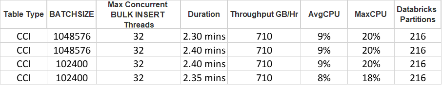
Please note that we are using default parallelism and partitions used by Azure Databricks and directly pushing the data to SQL Clustered Columnstore Indexed table. We have not manipulated any default configuration used by Azure Databricks. Irrespective of the BatchSize defined, all our tests were completed at approximately the same time.

The 32 concurrent threads loading the data into SQL DB is due to the size of provisioned Databricks cluster mentioned above. The cluster has maximum of 8 worker nodes with 4 cores each i.e., 8*4 = 32 cores capable of running a maximum of 32 concurrent threads at max.

A Look at Row Groups

For table in which we inserted the data with BATCHSIZE 1,048,576, here are the number of row groups created in SQL:

Total number of row groups:

SELECT COUNT(1) 
FROM sys.dm_db_column_store_row_group_physical_stats 
WHERE object_id = OBJECT_ID('largetable110M_1048576')
216

Quality of row groups:

SELECT * 
FROM sys.dm_db_column_store_row_group_physical_stats 
WHERE object_id = OBJECT_ID('largetable110M_1048576')

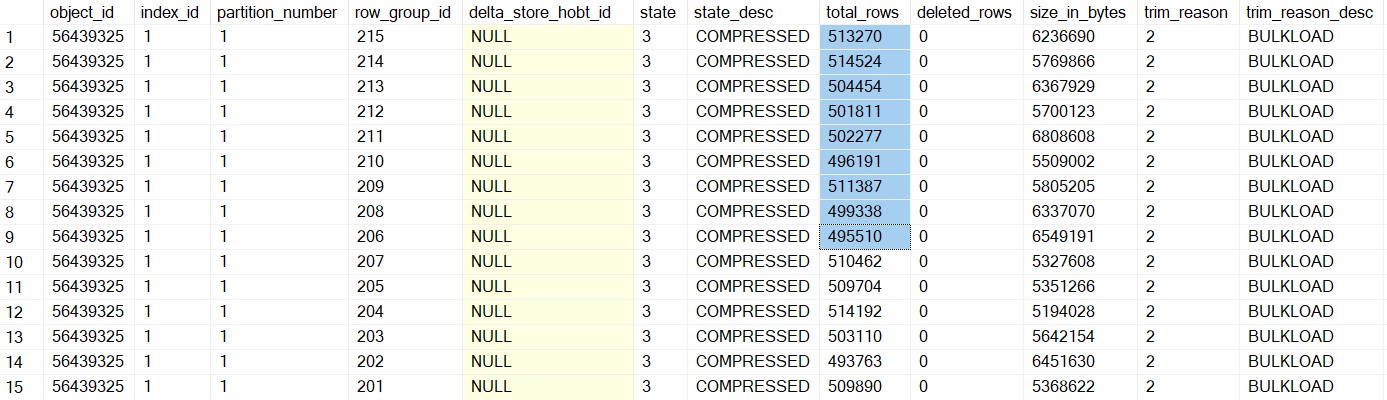
In this case, we have only one delta store with OPEN state (total_rows = 3810) and 215 row groups which were in COMPRESSED state, and this make sense because if the batch size for the insert is > 102,400 rows, the data no longer ends up in the delta store, rather is inserted directly into a compressed rowgroup in columnar format. In this case, all the row groups in the COMPRESSED state have >102,400 records. Now, the questions regarding row groups are:

1. Why do we have 216 row groups?
2. Why do each row group have a different number of rows in them when our BatchSize was set at 1,048,576?

Please note that each row group has data which is approximately equal to 500,000 records in the above result set.

The answer to both these questions is the way Azure Databricks spark engine partitions the data and controls the number of records getting inserted into row groups of Clustered Columnstore Index. Let’s have a look at the number of partitions created by Azure Databricks for the data set in question:

# Get the number of partitions before re-partitioning
print(df_gl.rdd.getNumPartitions())
216

# Number of records in each partition
from pyspark.sql.functions  
import spark_partition_id
df_gl.withColumn("partitionId", spark_partition_id()).groupBy("partitionId").count().show(10000)

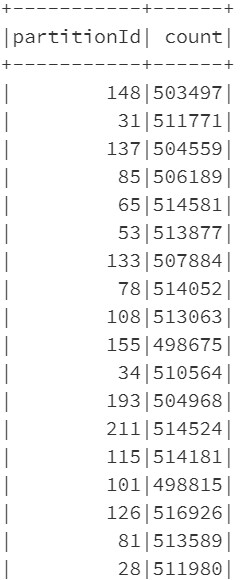
Comparing the number of records in spark partitions with the number of records in the row groups, you’ll see that they are equal. Even the number of partitions is equal to the number of row groups. So, in a sense, the BATCHSIZE of 1,048,576 is being overdriven by the number of rows in each partition.

sqldbconnection = dbutils.secrets.get(scope = "sqldb-secrets", key = "sqldbconn")
sqldbuser = dbutils.secrets.get(scope = "sqldb-secrets", key = "sqldbuser")
sqldbpwd = dbutils.secrets.get(scope = "sqldb-secrets", key = "sqldbpwd")
 
servername = "jdbc:sqlserver://" + sqldbconnection url = servername + ";" + "database_name=" + <Your Database Name> + ";"
table_name = "<Your Table Name>"

# Write data to SQL table with BatchSize 1048576
df_gl.write \
        .format("com.microsoft.sqlserver.jdbc.spark") \
        .mode("overwrite") \
        .option("url", url) \
        .option("dbtable", table_name) \
        .option("user", sqldbuser) \
        .option("password", sqldbpwd) \
        .option("schemaCheckEnabled", False) \
        .option("BatchSize", 1048576) \
        .option("truncate", True) \
        .save()

Row Group Quality

A row group quality is determined by the number of row groups and records per row group. Since a Columnstore index scans a table by scanning column segments of individual row group, maximizing the number of rows in each rowgroup enhances query performance. When row groups have a high number of rows, data compression improves which means there is less data to read from the disk. For the best query performance, the goal is to maximize the number of rows per rowgroup in a Columnstore index. A rowgroup can have a maximum of 1,048,576 rows. However, it is important to note that row groups must have at least 102,400 rows to achieve performance gains due to the Clustered Columnstore index. Also, remember that the maximum size of the row groups (1 million) may not be reached in every case, courtesy this document the rowgroup size is not just a factor of the max limit but is affected by the following factors.

• The dictionary size limit, which is 16 MB
• Insert batch size specified.
• The Partition scheme of the table since a rowgroup doesn’t span partitions.
• Memory Grants or memory pressure causing row groups to be trimmed.
• Index REORG being forced or Index Rebuild being run.

Having said that, it is now an important consideration to have row group size as close to 1 million records as possible. In this testing since the size of each row group is close to 500,000 records, we have two options to reach to the size of ~1 million records:

1. In spark engine (Databricks), change the number of partitions in such a way that each partition is as close to 1,048,576 records as possible,
2. Keep spark partitioning as is (to default) and once the data is loaded in a table run ALTER INDEX REORG to combine multiple compressed row groups into one.

Option#1 is quite easy to implement in the Python or Scala code which would run on Azure Databricks. The overhead is quite low on the Spark side.

Option#2 is an extra step which is needed to be taken post data loading and ofcourse, this is going to consume extra CPU cycles on SQL and add to the time taken for the overall loading process.

To keep the relevance of this article, let’s stick to Spark partitioning. Let’s now discuss more about spark partitioning and how it can be changed from its default values and its impact in the next section.

Spark Partitioning

The most typical source of input for a Spark engine is a set of files which are read using one or more Spark APIs by dividing into an appropriate number of partitions sitting on each worker node. This is the power of Spark partitioning where the user is abstracted from the worry of deciding number of partitions and the configurations controlling the partitions if they don’t desire. The default number of partitions which are calculated based on environment and environment settings typically work well for most of the cases. However, in certain cases a better understanding of how the partitions are automatically calculated and a user can alter the partition count if desired can make a stark difference in performance.

Note: Large Spark clusters can spawn a lot of parallel threads which may lead to memory grants contention on Azure SQL DB. You must watch out for this possibility to avoid early trim due to memory timeouts. Please refer this article for more details to understand how schema of the table and number of rows etc. also may have an impact on memory grants.

spark.sql.files.maxPartitionBytes is an important parameter to govern the partition size and is by default set at 128 MB. It can be tweaked to control the partition size and hence will alter the number of resulting partitions as well.

spark.default.parallelism which is equal to the total number of cores combined for the worker nodes.

Finally, we have coalesce() and repartition() which can be used to increase/decrease partition count of even the partition strategy after the data has been read into the Spark engine from the source.

coalesce() can be used only when you want to reduce the number of partitions because it does not involve shuffle of the data. Consider that this data frame has a partition count of 16 and you would want to increase it to 32, so you decide to run the following command.

df = df.coalesce(32)
print(df.rdd.getNumPartitions())

However, the number of partitions will not increase to 32 and it will remain at 16 because coalesce() does not involve shuffling. This is a performance-optimized implementation because you can get reduced partition without expensive data shuffle.

In case you want to reduce the partition count to 8 for the above example then you would get the desired result.

df = df.coalesce(8)
print(df.rdd.getNumPartitions())

This will combine the data and result in 8 partitions.

repartition() on the other hand would be the function to help you. For the same example, you can get the data into 32 partitions using the following command.

df = df.repartition(32)
print(df.rdd.getNumPartitions())

Finally, there are additional functions which can alter the partition count and few of those are groupBy(), groupByKey(), reduceByKey() and join(). These functions when called on DataFrame results in shuffling of data across machines or commonly across executors which result in finally repartitioning of data into 200 partitions by default. This default 200 number can be controlled using spark.sql.shuffle.partitions configuration.

Back to Data Loading

Now, knowing about how partition works in Spark and how it can be changed, it’s time to implement those learnings. In the above experiment, the number of partitions was 216 (by default) and it was because the size of the file was ~27 GB, so dividing 27 GB by 128 MB (which is maxPartitionBytes defined by Spark by default) gives 216 partitions.

Impact of Spark Re-partitioning

The change to be done to the PySpark code would be to re-partition the data and make sure each partition now has 1,048,576 rows or close to it. For this, first get the number of records in a DataFrame and then divide it by 1,048,576. The result of this division will be the number of partitions to use to load the data, let’s say the number of partitions is n. However, there could be a possibility that some of the partitions now have >=1,048,576 rows, hence, to make sure in each partition have rows <= 1,048,576 we take number of partitions as n+1. Using n+1 is also important in cases when the result of th division is 0. In such cases, you’ll have one partition.

Since the data is already loaded in a DataFrame and Spark by default has created the partitions, we now have to re-partition the data again with the number of partitions equal to n+1.

# Get the number of partitions before re-partitioning print(df_gl.rdd.getNumPartitions())
216 

# Get the number of rows of DataFrame and get the number of partitions to be used. 
rows = df_gl.count() 
n_partitions = rows//1048576  

# Re-Partition the DataFrame 
df_gl_repartitioned = df_gl.repartition(n_partitions+1)  

# Get the number of partitions after re-partitioning 
print(df_gl_repartitioned.rdd.getNumPartitions()) 
105 

# Get the partition id and count of partitions 
df_gl_repartitioned.withColumn("partitionId", spark_partition_id()).groupBy("partitionId").count().show(10000)  

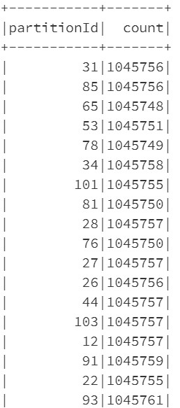
At this point, let’s write the data into SQL table again and verify the row group quality. This time the number of rows per row group will be close to the rows in each partition (a bit smaller than 1,048,576). Let’s see below:

Row Groups After Re-partitioning

SELECT COUNT(1) 
FROM sys.dm_db_column_store_row_group_physical_stats 
WHERE object_id = OBJECT_ID('largetable110M_1048576')
105

Quality of Row Groups After Re-partitioning

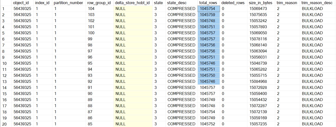
Essentially, this time the overall data loading was 2 seconds slower than earlier, but the quality of the row group was much better. The number of row groups was reduced to half, and the row groups are almost filled to their maximum capacity. Please note that there will an additional time consumed due to repartitioning of the data frame and it depends on the size of the data frame and number of partitions.

Disclaimer: Please note that you won’t always get 1 million records per row_group. It will depend on the data type, number of columns etc. along with factors discussed earlier – See trim_reason in sys.dm_db_column_store_row_group_physical_stats (Transact-SQL) – SQL Server | Microsoft Docs

Key Take Away

1. It is always recommended to use BatchSize while bulk loading data into SQL Server (be it CCI or Heap). However, in case Azure Databricks or any other Spark engine is used to load the data, the data partitioning plays a significant role to ascertain the quality of row groups in Clustered Columnstore index.
2. Data loading using BULK INSERT SQL command will honor the BATCHSIZE mentioned in the command, unless other factors affect the number of rows inserted into a rowgroup.
3. Partitioning the data in Spark shouldn’t be based on some random number, it’s good to dynamically identify the number of partitions and use n+1 as number of partitions.
4. Since a Columnstore index scans a table by scanning column segments of individual row groups, maximizing the number of records in each rowgroup enhances query performance. For the best query performance, the goal is to maximize the number of rows per rowgroup in a Columnstore index.
5. The speed of data loading from Azure Databricks largely depends on the cluster type chosen and its configuration. Also, note that as of now the Azure SQL Spark connector is only supported on Apache Spark 2.4.5. Microsoft has released support for Spark 3.0 which is currently in Preview, we recommend you to test this connector thoroughly in your dev\test environments.
6. Depending on the size of the data frame, number of columns, the data type etc. the time to do repartitioning will vary, so you must consider this time to the overall data loading from end-end perspective.

Photo by Ruiyang Zhang from Pexels

Sumit Senior Engineering Architect - Azure Data

Follow