Forecasting Service scale out with Jupyter Notebooks in Visual Studio Code

Kieran Brantner-Magee

Visual Studio Code has an extension for running Jupyter Notebooks, which is a great tool for those of us interested in data analytics as it simplifies our workflows. In this article, I will show how to consume Azure data in a Jupyter Notebook using the Azure SDK. The problem I will be demonstrating builds a predictive model to anticipate service scale-up, which is a common task for optimizing cloud spend and anticipating scale requirements.

To create the predictive model, I’ll need some data. My application is logging to Azure Application Insights, which then stores the data in Azure Blob Storage as a series of time-series log files.

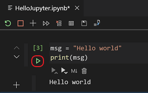
To start, you will need Visual Studio Code with the VSCode Python extension installed. When you run a Jupyter notebook for the first time, VSCode will prompt you to install necessary modules.

You can download the demo notebook and open it directly in VSCode. Jupyter notebooks intermesh code and documentation seamlessly, allowing for an interactive documentation experience.

The rest of this article walks through the Jupyter notebook. First, let’s bring in the packages we will need, including the Azure SDK that allows us to read the data, data manipulation, forecasting, and visualization packages.

import sys

# Azure SDK for storage and identity
!"{sys.executable}" -m pip install azure-storage-blob azure-identity
# Data manipulation
!"{sys.executable}" -m pip install pandas numpy sklearn
# Visualization
!"{sys.executable}" -m pip install matplotlib
# Tooling to perform ARIMA forecasts
!"{sys.executable}" -m pip install pmdarima
# Needed to run the notebook
!"{sys.executable}" -m pip jupyter notebook

This uses an odd quoting to ensure that the application supports paths with spaces in them. If you bump into permissions issues, you may be using a system installed version of Python and do not have permissions to install packages for global use. You can install Python in a user-controlled location instead, and set your Jupyter kernel accordingly.

Loading the data

Next, we need to load the data from Azure Blob Storage, which means dealing with authentication. Azure Identity provides a handy class called the DefaultAzureCredential that simplifies authentication. This lets you log in to Azure with a number of different utilities, including (if necessary) an interactive browser.

from azure.identity import DefaultAzureCredential

credential = DefaultAzureCredential(True)

We can now access the storage account where the logs are stored. In this example, I’m using an Azure App Service that is logged to Application Insights. Application Insights is configured to continuously export log and telemetry data to Azure Blob Storage. The methodology can be applied to any similarly shaped data.

First, create a connection to the storage account:

# Name of the Azure Storage account
azure_storage_account = 'REPLACE_ME'
# Name of the Container holding the data
azure_storage_container = 'REPLACE_ME'
# Base path for the blobs within the container
azure_storage_path = 'REPLACE_ME'

from azure.storage.blob import BlobServiceClient

storage_account_url = "https://{}.blob.core.windows.net".format(azure_storage_account)
storage_client = BlobServiceClient(storage_account_url, credential)

We can now use the storage_client to enumerate and fetch the logs stored in blobs within the container. If you receive an authentication error in this section, check that the user or service principal being used has “Blob Data Owner” permissions to the storage account; “Owner” is not sufficient by itself. Refer to the Azure documentation for more information.

import json
import pandas
from datetime from datetime, timedelta

def extract_requests_from_container(client, blob_path, container_name, start_time=None, end_time=None):
    '''App Insights stores data in a series of folders (Metrics, Requests, etc.) within a container.
    This function enumerates the blobs within the Requests folder, extracting the JSON formatted
    request logs and storing their counts and timestamps to a dataframe.'''

    data = pandas.DataFrame(columns=['count'])
    container = client.get_container_client(container_name)
    blob_list = container.list_blobs(blob_path + '/Requests/')
    for blob in blob_list:
        body = container.download_blob(blob.name).readall().decode('utf8')
        for request_string in body.split('\n'):
            try:
                request = json.loads(request_string)
                # Convert from string to date
                event_time = datetime.strptime(request['context']['data']['eventTime'][:-2], r'%Y-%m-%dT%H:%M:%S.%f')
                if (event_time < start_time or event_time > end_time):
                    continue
                count = sum(r['count'] for r in request['request'])
                data.loc[event_time] = count
            except:
                continue
    return data

data = extract_requests_from_container(storage_client, azure_storage_path, azure_storage_container, 
    datetime.utcnow() - timedelta(hours=3), datetime.utcnow())

This code iterates through all the blobs in the ‘/Requests/’ folder, reads the JSON from the file, and creates a dataframe with the count of requests.

Preparing the data

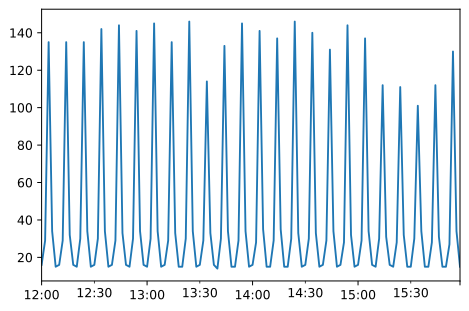
Now that we have some raw data, we can aggregate it into a useful granularity to do forecasting. The initial data set is per-event. It would be more useful to have the data bucketed by a timespan that allows us to see the underlying pattern we’re hoping to model. For our data, we’ll use 2 minute buckets. This may naturally differ with other datasets, the but goal is the same: produce a continuous and non-sparse representation of the desired load trend, smoothing over short-term variance without losing too much signal.

grouped_data = data.groupby(pandas.Grouper(freq='2Min')).agg({'count'})
grouped_data.plot(legend=False)

Note how easy it is to embed visualizations within a Jupyter Notebook!

Modeling the data

Now that we have a reasonably clean data set to work with, let’s apply forecasting techniques to provide a window into future behavior. We will use an ARIMA model. The ARIMA model is an algorithm that uses historical data to determine the underlying seasonality coupled with underlying moving averages for prediction. If you are familiar with regression-based approaches (such as linear or polynomial algorithms), ARIMA can better capture higher order behavior by leveraging seasonal look-backs, making it a useful tool for the sort of data patterns we see in service infrastructure.

There is often a lot of analysis in determining the proper parameters to an ARIMA model; something that is outside the scope of this article. We’ll utilize an auto-arima package that attempts to determine the optimal structure of the model for us.

from pmdarima import auto_arima
from pmdarima.model_selection import train_test_split
from matplotlib import pyplot
import numpy

train, test = train_test_split(grouped_data)
model = auto_arima(train, suppress_warnings=True)

# Visualize the results
forecast = model.predict(test.shape[0])
x = numpy.arange(grouped_data.shape[0])
pyplot.plot(x[:len(train)], train, c='blue')
pyplot.plot(x[:len(train):], forecast, c='green')
# to compare vs. actual results, uncomment next line
# pyplot.plot(x[len(train):], test, c='orange')
pyplot.show()

The forecast captures the primary data trend nicely. We can add the left-out test data to the chart to compare between the forecast and actual data.

It is normal to not include all historical data when training your model. Including all historical data may result in overfitting if the behavior of the data changes subtlely. Finding a balance between “enough data to capture the trend” and “not enough to overfit” is an important point to consider. Jupyter notebooks can help by easily providing an environment to do this analysis, and can give inspiration for automation techniques.

Use Azure Storage to iterate and automate

Now that we have a promising model, we need to ensure it does not regress. A common pattern for this is to store the hyperparameters and model outcomes in a persisted data store such as Azure Storage. We’ll reuse the client that we used earlier. The credential you are using will need the “Blob Data Writer” permission to write back to Azure Storage.

First, let’s capture some metrics to denote the current state of the model:

from sklearn.metrics import mean_squared_error

# Root mean squared error - a common method for observing the delta between forecast and actual
rmse = numpy.sqrt(mean_squared_error(test, forecast))
# Akaike's information criterion, a measure that also folds the "simplicity" of the model into the score
aic = model.aic()
# When the last forecast was made
forecast_time = test.index[-1]
# Parameters for the model
params = model.params()

Now, store these in an Azure Storage blob. This same information could be stored in any store; for example, CosmosDB, Table storage, or an SQL database.

from azure.core.exceptions import ResourceExistsError

# The container that will hold the output data
output_container_name = 'REPLACE_ME'

# Create the container if it doesn't exist
try:
    storage_client.create_container(output_container_name)
except ResourceExistsError:
    print("Warning: Container already exists")

# Upload data to a blob
import json
blob_client = storage_client.get_blob_client(output_container_name, str(forecast_time))
try:
    blob_client.upload_blob(json.dumps({
        'rmse': rmse,
        'aic': aic,
        'forecast_time': str(forecast_time),
        'params', list(params)
    }))
except ResourceExistsError:
    print("Warning: Blob already exists")

We can then take steps similar to fetching the initial log data above to pull the model logs for inspection; for instance, to watch for a regression in model performance:

container = storage_client.get_container_client(output_container_name)
blob_list = container.list_blobs()
for blob in blob_list:
    body = json.loads(container.download_blob(blob.name).readall().decode('utf8'))
    print(body)

Conclusion

During this article, we’ve demonstrated how to consume semi-structured data, transform it into a useful form, perform analytics, and publish those results for further use. While this is a tightly scoped example, this pattern is quite close to the structure of commonly used systems for understanding and acting on time-series data. We hope we have also shown the utility of Jupyter Notebooks for interactive data exploration and communication, coupled with the capabilities of Azure Storage for data persistence.

Follow us on Twitter at @AzureSDK. We’ll be covering more best practices in cloud-native development as well as providing updates on our progress in developing the next generation of Azure SDKs.

Kieran Brantner-Magee Software Engineer, Azure SDK

Follow