
Hospitals around the world regularly work towards improving the health of their patients as well as ensuring there are enough resources available for patients awaiting care. During these unprecedented times with the COVID-19 pandemic, Intensive Care Units are having to make difficult decisions at a greater frequency to optimize patient health outcomes.
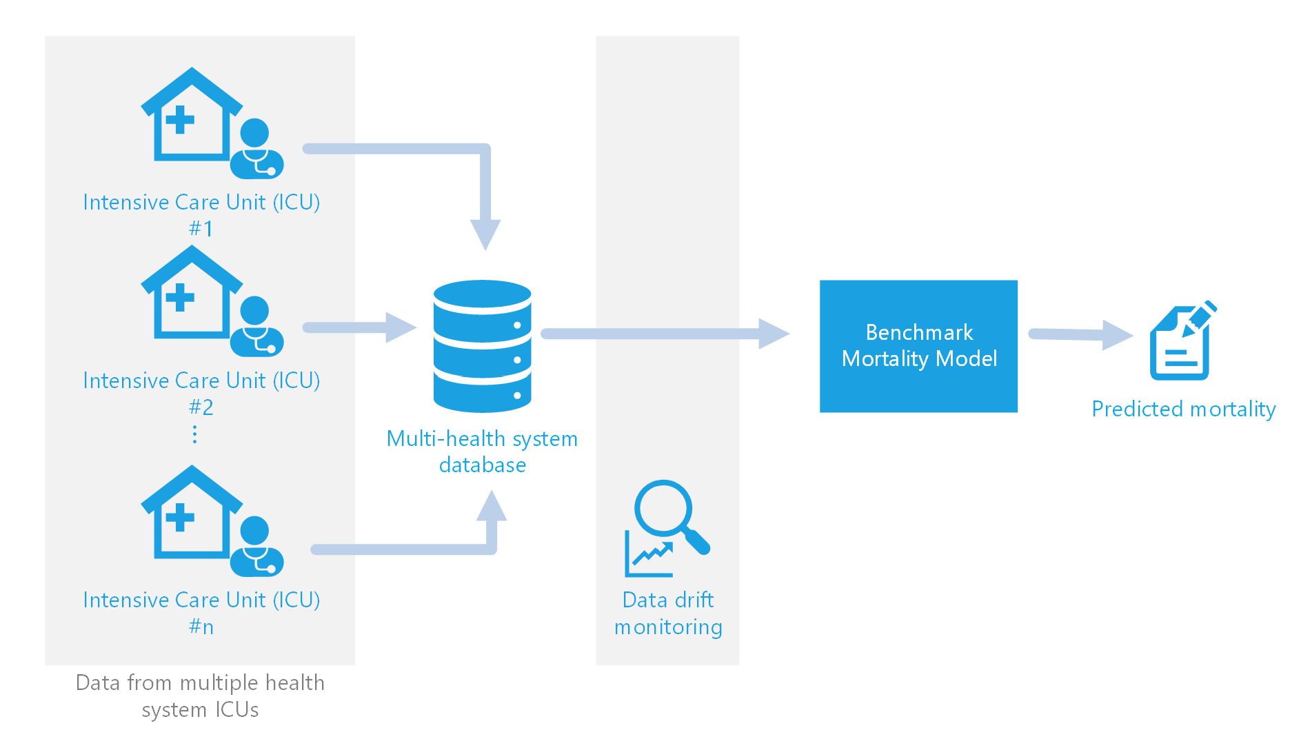
The continuous collection of biometric and clinical data throughout a patient’s stay enables medical professionals to take a data-informed, holistic approach to clinical decision making.

In some cases, a Machine Learning model may be used to provide insight given the copious amount of data coming in from various monitors and clinical tests per patient. The Philips Healthcare Informatics (HI) team uses such data to build models predicting outcomes such as likelihood of patient mortality, necessary length of ventilation, and necessary length of stay. In the case of the recent collaboration between us in Microsoft Commercial Software Engineering (CSE) and the Philips HI team, we focused on developing an MLOps solution to bring the Philips benchmark mortality model to production. This benchmark mortality model predicts the risk of patient mortality on a quarterly basis as an evaluation metric for individual ICU performance.
Since the model uses such a large amount of information from various sources, it is imperative that the quality of the incoming data be monitored to catch any changes that may affect model performance. Manually investigating unexpected changes and tracking down the cause of the data problems takes valuable time away from the data science team at Philips working on the mortality and other models.
In this blog post, we cover our approach to establishing a data drift monitoring process for multifaceted clinical data in the Philips eICU network, including example code.
Challenges and Objectives
The aim of this collaboration was to integrate MLOps into the Philips team’s workflow to improve their experience with moving code from development to production, as well as to enable scalability and to increase overall efficiency of their system. MLOps, also known as DevOps for Machine Learning, is a set of practices that enable automation of aspects of the Machine Learning lifecycle and help ensure quality in production (see the Resources section at the end of this post). Various workstreams of the solution focused on components of MLOps integration, including monitoring model performance and fairness.
One of our key objectives was to develop a data drift monitoring process and integrate it into production such that potential changes in model performance could be caught before re-running the time-intensive and computationally expensive model training pipeline, which is run quarterly to generate a performance report for each ICU or acute unit monitored by an enterprise eICU program.
Regarding data drift monitoring, we aimed to:
- Create distinct pipelines for input data monitoring and model training such that data drift monitoring could be performed more frequently and separately from model training.
- Perform both schema validation and distribution drift monitoring for numerical and categorical features to bring attention to noteworthy changes in data.
- Ensure data drift monitoring results are easily interpretable and provide useful insight on changes in the data.
- Structure a scalable and secure solution such that the framework established can accommodate additional models and datasets in the near future.
What is Data Drift?
Drift, in the context of this project, involves shifts or changes in the format and values of data being fed as input into the mortality model. In general, data drift detection can be used to alert data scientists and engineers to changes in the data and can also be used to automatically trigger model retraining. In this project, we perform data drift monitoring to catch potential issues before running the time intensive model retraining. We separate data drift into two streams, schema validation and distribution drift monitoring.
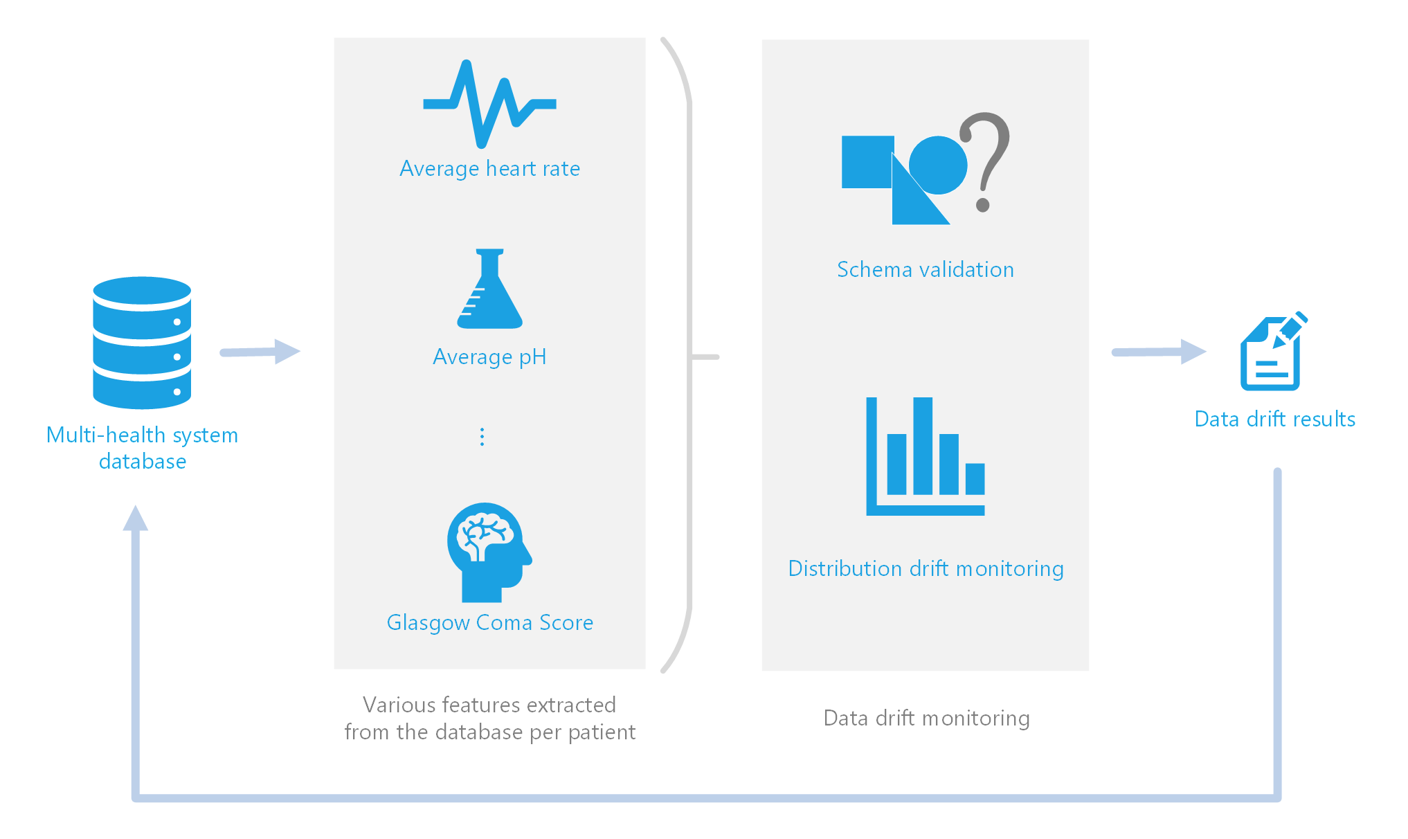
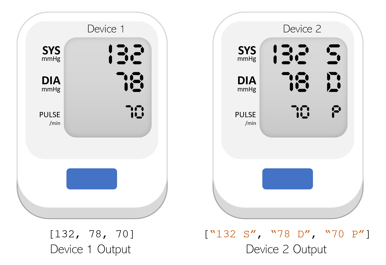
Schema drift involves changes in the format or schema of the incoming data. For example, let’s consider the case of an ICU using a new machine for recording blood pressure. This new machine outputs diastolic and systolic blood pressure as two strings (e.g., [“120 S”, “80 D”]) instead of as two integers like with the previous machine (e.g., [120, 80]). This unexpected change in format could lead to an error when attempting to retrain the model. Implementing automatic schema validation allows the team to quickly catch when breaking changes are introduced into the model training dataset.
Distribution drift, also known as virtual concept drift or covariate shift, involves change in the overall distribution of data within each feature over time. For example let’s consider the case of one ICU’s blood pressure monitors malfunctioning or recalibrated, leading to reporting diastolic blood pressure as 25 points higher and systolic blood pressure as 18 points lower consistently. This would be important to catch as the change may not cause the model to fail, but it may negatively impact the performance of the model for patients in this ICU.
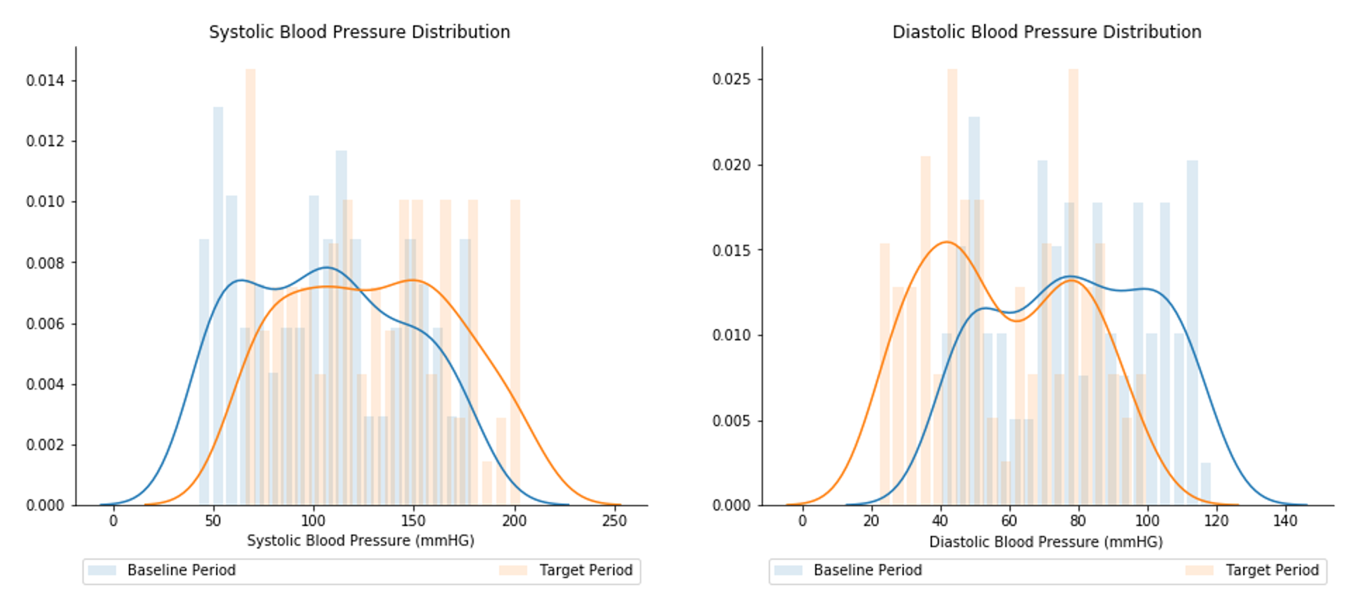
Distribution drift is calculated as the difference between a baseline and target distribution. For any given feature (e.g., diastolic blood pressure), the baseline distribution is a set of values for that feature from a historical time window (e.g., from January 1, 2018 to December 31, 2018) which the target distribution will be compared against. Likewise, the target distribution is a set of values for the given feature from a more recent time window (e.g., from January 1, 2019 to December 31, 2019). Figure 4 illustrates example baseline and target distributions for diastolic and systolic blood pressure.
The difference in distributions for each feature is measured and evaluated as statistically significant using Kolmogorov-Smirnov tests, as available through the Python alibi-detect library. If the distributions are considered statistically significant, the feature is marked as having statistically significant drift.
It is important to note that while some feature drift is seasonal or expected, data scientists should be aware of changes in the data that could affect model performance. Staying abreast of these changes, data scientists can communicate with hospital staff early on how to address any issues before the ICU performance reports are created.
While the above examples do not appear as a major issue if blood pressure were the only feature used in the model, the model takes in data for many features across many hospitals and health systems. It would be impractical to manually inspect all the data to understand why the model is failing to retrain or why the model is performing worse after retraining.
Solution
Our solution needed to be scalable, repeatable, and secure. As a result, we built our solution on Azure Databricks using the open source library MLflow, and Azure DevOps.
For the data drift monitoring component of the project solution, we developed Python scripts which were submitted as Azure Databricks jobs through the MLflow experiment framework, using an Azure DevOps pipeline. Example code for the data drift monitoring portion of the solution is available in the Clinical Data Drift Monitoring GitHub repository.
Table 1 details the tools used for building the data drift monitor portion of the solution.
| Tool Used | Reason | Resources |
| Azure Databricks | Great computational power for model training and allows for scalability. | Azure Databricks, Azure Databricks documentation |
| SQL Server | The healthcare data was already being stored in a SQL server database. No need to move the data. | Accessing SQL databases on Databricks using JDBC |
| Alibi-detect | Established Python package with data drift detection calculation capabilities. | Alibi-detect GitHub repository |
| MLflow | Established open source framework for tracking model parameters and artifacts. | MLflow overview |
| Azure DevOps | All-inclusive service for managing code and pipelines for the full DevOps lifecycle. | What is Azure DevOps?, Azure DevOps documentation |
Table 1. Tools used were selected to accommodate the whole solution, including data drift monitoring. An important criterion in our tool selection was integration to the solution as a whole.
With our MLOps approach, the data drift monitor code is continuously integrated into the solution and does not exist as isolated code. In this post, we will first cover the general structure of the MLOps code and then move into the strictly drift monitoring code.
Note, for this blog post and in the example code, we use The New York Times open source COVID-19 cases by county dataset to demonstrate data drift monitoring instead of sensitive clinical data.
General Workflow
Before running the data drift monitoring code, we needed to set up the Azure Databricks workspace connection to where all computation would take place (Figure 5). For guidance on how to create a shared resource group connected to an Azure Databricks workspace, see this getting started README on this blog post repository. For guidance on creating an Azure Databricks workspace, see the Azure Databricks documentation.

After creating the shared resource group connected to our Azure Databricks workspace, we needed to create a new pipeline in Azure DevOps that references the data drift monitoring code. In our data_drift.yml pipeline file, we specify where the code is located for schema validation and for distribution drift as two separate tasks.
  - task: Bash@3
    displayName: Execute Data Drift Project (schema validation)
    inputs:
      targetType: "inline"
      script: |
        python scripts/submit_job.py \
          --projectEntryPoint validation \
          --projectPath projects/$(PROJECT_NAME)/ \
          --projectExperimentFolder $(MODEL_WORKSPACE_DIR)/data_drift \
    env:
      MLFLOW_TRACKING_URI: databricks
      MODEL_NAME: "$(PROJECT_NAME)datadrift"
      MODEL_ID: $(MODEL_ID)
      DATA_PATH: $(DATA_PATH)
      FEATURES: $(FEATURES)
      DATETIME_COL: $(DATETIME_COL)
      GROUP_COL: $(GROUP_COL)
      BASELINE_START: $(BASELINE_START)
      BASELINE_END: $(BASELINE_END)
      TARGET_START: $(TARGET_START)
      TARGET_END: $(TARGET_END)
      P_VAL: $(P_VAL)
      OUT_FILE_NAME: $(OUT_FILE_NAME)
During pipeline creation, we specify pipeline variables that serve as parameters for the various drift-related Python scripts (Table 2) that can also be seen in the code snippet above. The default values in the table coincide with the open source The New York Times COVID-19 cases by county dataset we use in the example code.
| Variable Name | Default Value | Description |
| BASELINE_END | 2020-05-31 | End date of the baseline period in YYYY-MM-DD format. |
| BASELINE_START | 2020-01-21 | Start date of the baseline period in YYYY-MM-DD format. |
| DATA_PATH | https://raw.githubusercontent.com/nytimes/covid-19-data/master/us-counties.csv | Location of data (either local path or URL). |
| DATETIME_COL | date | Name of column containing datetime information. |
| FEATURES | fips,cases,deaths | List of features to perform schema validation for, separated by commas with no spaces. |
| GROUP_COL | state | Name of column to group results by. |
| MODEL_ID | 1 | Appropriate model ID number associated with the data we are performing drift monitoring for (see mon.vrefModel). |
| OUT_FILE_NAME | results.json | Name of .json file storing results. |
| P_VAL | 0.05 | Threshold value for p-values in distribution drift monitoring. Values below the threshold will be labelled as significant. |
| TARGET_END | 2019-08-27 | End date of the target period in YYYY-MM-DD format. |
| TARGET_START | 2019-08-01 | Start date of the target period in YYYY-MM-DD format. |
Table 2. The data drift monitoring pipeline allows the user to set parameters (variable values) that are appropriate for any particular given run. These values are used by the data drift monitoring Python scripts.
Each variable was set such that whoever triggers the pipeline can override the default values with values more appropriate for the specific run instance (e.g., changing the target start and end dates) (Figure 6). For further guidance on creating this pipeline, see mlops_example_data_drift_project.md on this blog post repository.

With the Azure Databricks workspace and the pipeline set up, let’s look at the code our pipeline references.
DriftCode
-  common (dir)
-  distribution (dir)
     - parameters.json.j2
     - [distribution drift monitoring script]
-  validation (dir)
     - parameters.json.j2
     - [schema validation scripts]
-  cluster.json.j2
-  MLProject
-  project_env.yaml
With the MLflow framework, the environment, parameters, and script calls are all referenced in the MLProject file. We organize code specific to schema validation into the “validation” folder and code specific to distribution drift to the “distribution” folder, which we will discuss later in this post.
In order to use Databricks for computation, we define our cluster, which our MLflow project will be submitted to as a Databricks job.
{
  "spark_version": "7.0.x-scala2.12",
  "num_workers": 1,
  "node_type_id": "Standard_DS3_v2",
  "spark_env_vars": {
    "MODEL_NAME": "{{MODEL_NAME}}"
    {% if AZURE_STORAGE_ACCESS_KEY is defined and AZURE_STORAGE_ACCESS_KEY|length %}
      ,
      "AZURE_STORAGE_ACCESS_KEY": "{{AZURE_STORAGE_ACCESS_KEY}}"
    {% endif %}
  }
}
Because the data drift monitoring code requires specific dependencies that other workstreams in the overall solution may not need, we specify an Anaconda environment for all the Python code to run on.
---
name: drift
channels:
  - defaults
  - anaconda
  - conda-forge
dependencies:
  - python=3.7
  - pip:
      - environs==8.0.0
      - alibi-detect==0.4.1
      - mlflow==1.7.0
      - tensorflow==2.3.0
      - cloudpickle==1.3.0
The Data Drift Monitoring Code
The first step to detecting either changes in schema or distribution is loading the data. In the project with Philips, we connected to a SQL server to access the data using a combination of PySpark and JDBC.
import os
import numpy as np
from pyspark.sql import SparkSession
from environs import Env

spark: SparkSession = SparkSession.builder.getOrCreate()
def get_sql_connection_string(port=1433, database="", username=""):
    """ Form the SQL Server Connection String

    Returns:
        connection_url (str): connection to sql server using jdbc.
    """
    env = Env()
    env.read_env()
    server = os.environ["SQL_SERVER_VM"]
    password = os.environ["SERVICE_ACCOUNT_PASSWORD"]

    connection_url = "jdbc:sqlserver://{0}:{1};database={2};user={3};password={4}".format(
        server, port, database, username, password
    )

    return connection_url


def submit_sql_query(query):
    """ Push down a SQL Query to SQL Server for computation, returning a table

    Inputs:
        query (str): Either a SQL query string, with table alias, or table name as a string.

    Returns:
        Spark DataFrame of the requested data
    """
    connection_url = get_sql_connection_string()
    return spark.read.jdbc(url=connection_url, table=query)
For simplicity, in this example we do not connect to a SQL server but instead load our data from a local file or URL into a Pandas data frame. Here, we explore the open source The New York Times COVID-19 dataset which includes FIPS codes (fips), cases, and deaths by county in the United States of America over time.
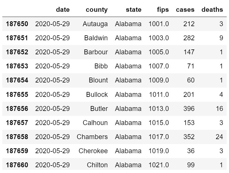
Although not as complex as the data used to estimate optimal ICU stay length or mortality for the Philips model, this simple dataset allows us to explore data drift monitoring with minimal data wrangling and processing.
Schema Validation
Part of the drift monitoring pipeline involves checking if the schema of the data is as expected. In our solution, this schema validation is written as a separate script for each feature (i.e., fips, cases, deaths) followed by an assertion script which causes the pipeline to fail if any of the features present invalid schema.
The following is an example of the nature of custom schema validation for a particular feature.
"""
Assumptions for cases:
    - Values are integers
    - Values are non-negative
"""
for group_value in group_values:
    # ---------------------------------------------------
    # Get unique values in the column (feature) of interest
    # ---------------------------------------------------
    feature_values = get_unique_vals(df, feature, group_col, group_value)

    # Initialize variable to keep track of schema validity
    status = "valid"

    # Validate feature schema
    for val in feature_values:

        # Continue this loop until you hit an invalid
        # This prevents from only saving the last value's status
        if status == "valid":

            # Check if value is a float
            if type(val) in [int, np.int64]:
                if val < 0:
                    status = "invalid: value must be non-negative"
                else:
                    status = "valid"
            else:
                status = "invalid: value not an int"

        # Update dictionary
        output_dict["schema_validation"][group_col][group_value].update(
            {feature: {"status": status, "n_vals": len(feature_values)}}
        )
Note that the specific logic will vary depending on the particular assumptions for the given feature.
With each feature schema check, validation results are written to a .json file which is read in as a dictionary in the assertion script.
def search_dict_for_invalid(group_col, group_values, features, results, invalids):
    """ Search dictionary for features with invalid schema

    Inputs:
        group_col (str): Name of column to group results by.
        group_values (str): Names of specific groups in group_col.
        features (list of str): List of features that will be monitored.
        results (dict): Dictionary containing schema validation results and metadata.
        invalids (list): List of strings containing information about which features are invalid.

    Return:
        invalids (list): List of strings containing information about which features are invalid.
    """
    for group_value in group_values:
        for feature in features:
            status = results["schema_validation"][group_col][group_value][feature][
                "status"
            ]
            if status.lower() != "valid":
                invalids.append(
                    "{0}: {1}, {2} invalid".format(group_col, group_value, feature)
                )

    return invalids
If the schema for any of the features is determined “invalid”, the assertion call in the assertion script will throw an error.
Distribution Drift
The other half of the drift monitoring pipeline calculates distribution drift within each of the features over the user-specified baseline and target periods. This drift is calculated using Kolmogorov-Smirnov (K-S) tests implemented through the alibi-detect Python library. We decided to use K-S tests as they account for multiple comparisons, which is relevant for when running statistical tests on multiple features of interest (i.e., fips, cases, deaths). In addition, drift detection through alibi-detect allows for seamless handling of categorical data and has the potential to predict malicious drift through adversarial drift detection.
from alibi_detect.cd import KSDrift
import pandas as pd
import numpy as np
import datetime
import argparse
import decimal
import mlflow
import os
import sys
from environs import Env
...
# ---------------------------------------------------
# Drift detection
# ---------------------------------------------------
X_baseline = df_baseline[features].dropna().to_numpy()
X_target = df_target[features].dropna().to_numpy()

if X_target.size == 0:
    return output_df

# Initialize drift monitor using Kolmogorov-Smirnov test
# https://docs.seldon.io/projects/alibi-detect/en/latest/methods/ksdrift.html
cd = KSDrift(p_val=p_val, X_ref=X_baseline, alternative="two-sided")

# Get ranked list of feature by drift (ranked by p-value)
preds_h0 = cd.predict(X_target, return_p_val=True)
drift_by_feature = rank_feature_drift(preds_h0, features)
With this, we set the p-value threshold to the threshold value set in the pipeline run (0.05 by default). This allows us to automatically label distribution drift for specific features as statistically significant or not in our results.
Note, in this example with The New York Times COVID-19 by county dataset, we do not have any categorical variables but the alibi-detect implementation of K-S tests allows us to run drift detection as if they were numerical without having to apply any processing.
Accessing Monitoring Results
To view the results of the schema validation and distribution drift monitoring, we view the resulting files written from the schema validation and distribution drift tasks.
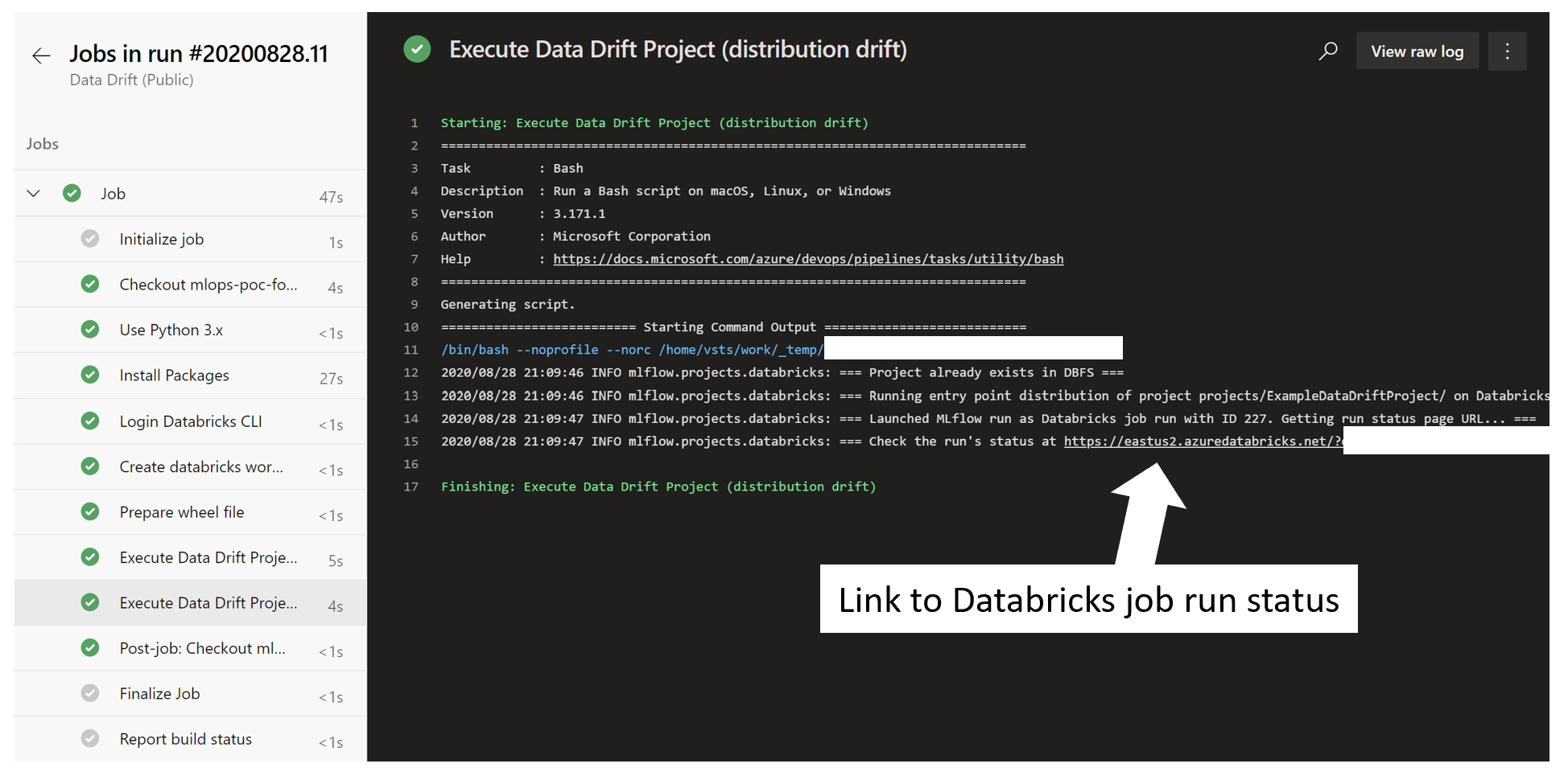
Status of the schema validation and distribution drift MLflow experiments (submitted as Databricks jobs) may be viewed in links provided for the respective tasks in the Azure DevOps pipeline run (Figure 8).
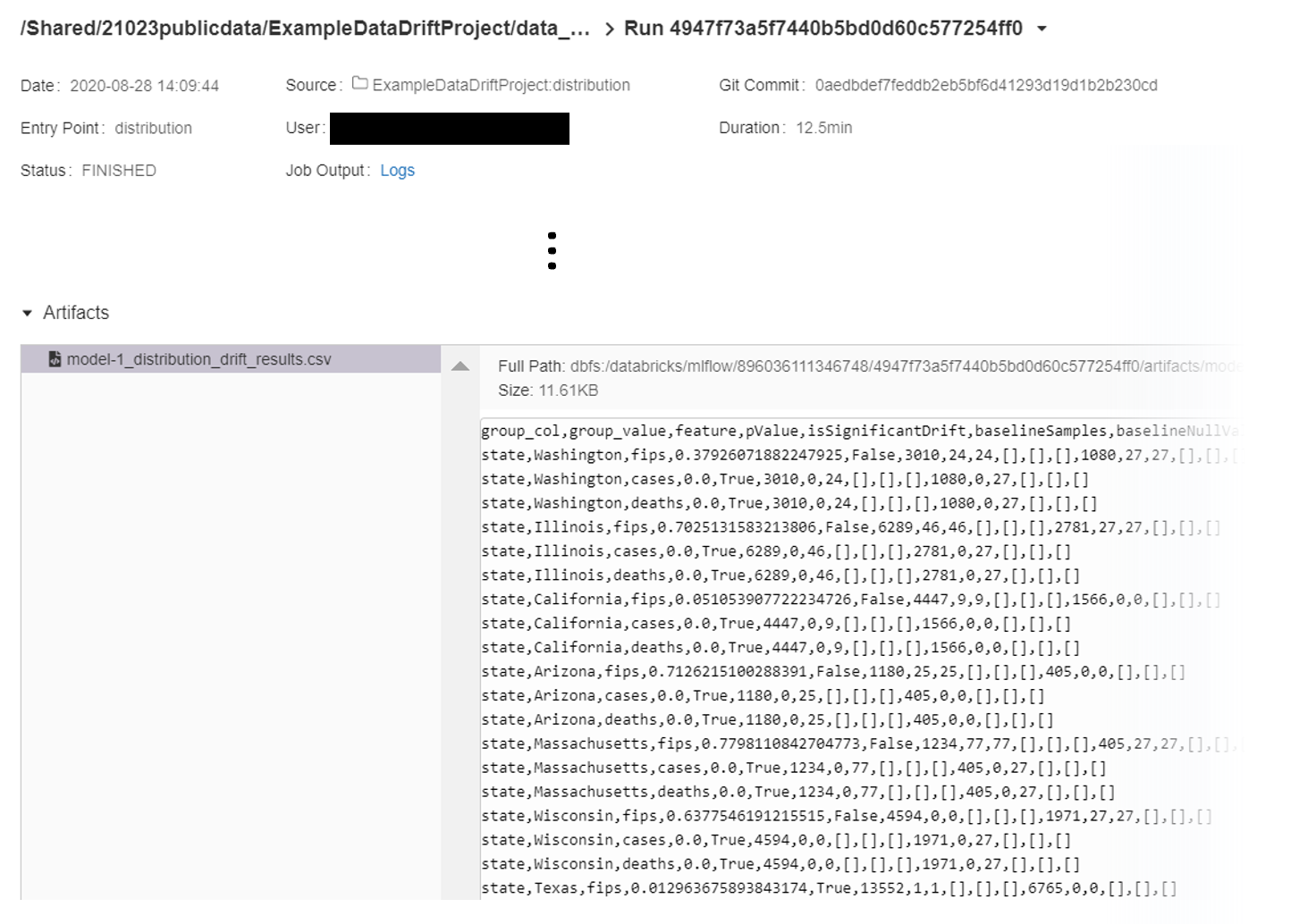
We can set the artifacts to be written either to Azure blob storage or directly to the Databricks file system (dbfs). In this example, we write directly to dbfs for easy access through the job summary in the Databricks workspace.
However, if you would like to instead write the files to Azure blob storage, you can uncomment/comment the appropriate lines in data_drift.yml to automatically route artifact uploading to blob.
# Keep the below line commented out if using dbfs, otherwise uncomment if using blob storage instead
# - group: mlops-vg-storage
...
# Optional to write artifacts to blob storage
# Comment out if using dbfs instead of blob storage
# AZURE_STORAGE_ACCESS_KEY: $(AZURE_STORAGE_ACCESS_KEY)
# AZURE_STORAGE_ACCOUNT_NAME: $(AZURE_STORAGE_ACCOUNT_NAME)
# AZURE_STORAGE_CONTAINER_NAME: $(AZURE_STORAGE_CONTAINER_NAME)
Now looking into the artifacts, we see a .json and .csv file for the schema validation and a single .csv file for the distribution drift results.
The .json and .csv for schema validation contain the same information but are formatted slightly differently. We decided to output results as a .csv for both schema validation and for distribution drift to easily write to SQL tables for the Philips project due to their tabular structure. The .json file is a bit easier to visually parse for anyone interested in looking directly at the results without writing specific queries.

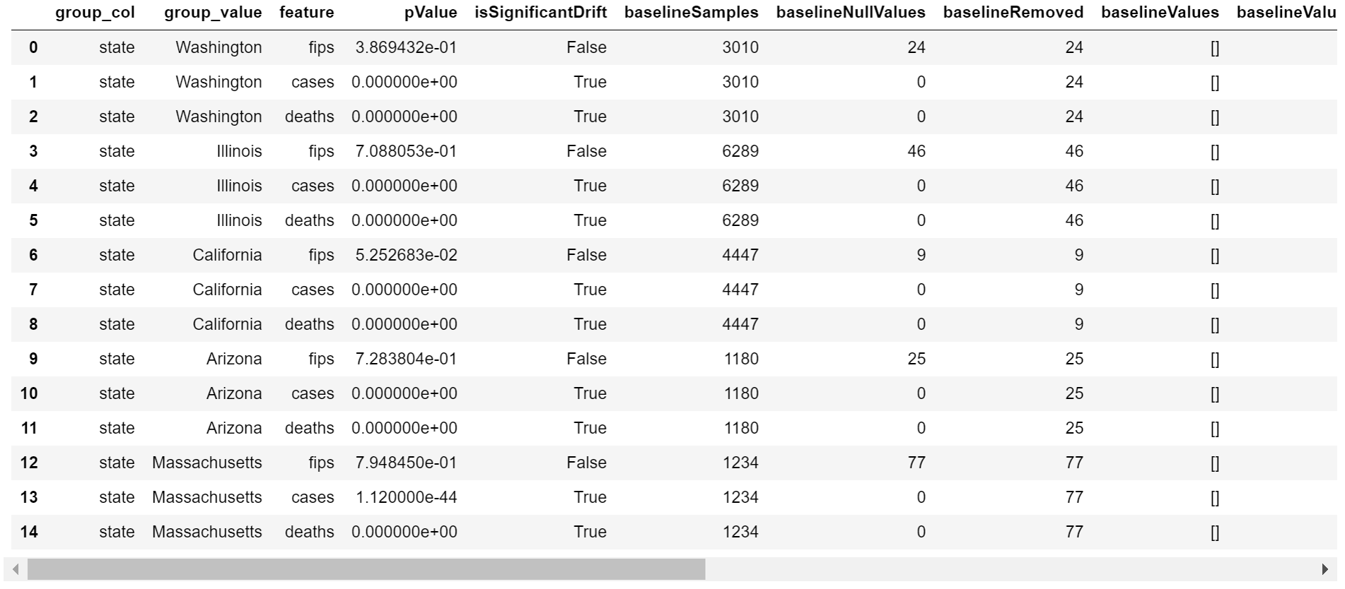
For distribution drift, results are organized into multiple columns which also allow for insight into categorical variable distribution changes (Table 3).
| Column Name | Type | Description |
| group_col | string | Name of column used to group results (e.g., “state”). |
| group_value | string | Value in group_col (e.g., “Nebraska”). |
| feature | string | Name of feature that drift detection is being run on (e.g., “cases”). |
| pValue | float | Threshold set for determining significance for Kolmogorov-Smirnov test on a given feature. |
| isSignificantDrift | boolean | True or False on whether drift detection on a feature results in a p-value below the pValue threshold. |
| baselineSamples | integer | The number of samples present in the baseline. |
| baselineNullValues | integer | The number of null values in the baseline for this specific feature. |
| baselineRemoved | integer | The number of rows removed in the baseline, based on presence of null in all features. |
| baselineValues | string | If the feature is categorical, a list of all values present in the baseline (e.g., [yes, no, maybe]) |
| baselineValueCounts | string | If the feature is categorical, a list of counts for all values present in the baseline (e.g., [60, 30, 10]) |
| baselineValuePercentages | string | If the feature is categorical, a list of proportions for all values present in the baseline (e.g., [0.6, 0.3, 0.1]) |
| targetNullValues | integer | The number of null values in the target for this specific feature. |
| targetRemoved | integer | The number of rows removed in the target, based on presence of null in all features. |
| targetValues | string | If the feature is categorical, a list of all values present in the target (e.g., [yes, no, maybe]) |
| targetValueCounts | string | If the feature is categorical, a list of counts for all values present in the target (e.g., [60, 30, 10]) |
| targetValuePercentages | string | If the feature is categorical, a list of proportions for all values present in the target (e.g., [0.6, 0.3, 0.1]) |
Table 3. Distribution drift monitoring results are stored in a table where each row contains the results for a particular group’s feature. In the case of The New York Times COVID-19 dataset, a state or county can be set as the “group” and fips, cases, or deaths are the possible features.
The columns baselineValues, baselineValueCounts, baselineValuePercentages, targetValues, targetValueCounts, and targetValuePercentages are all empty in this example as they are meant to contain data for categorical variables (Figure 11).
Conclusion
Data drift monitoring is a key part of model maintenance that allows for data scientists to identify changes in the source data that may be detrimental to model performance before retraining the model.
In the context of the Philips Healthcare Informatics (HI) / Microsoft collaboration, the implementation of data drift monitoring into their MLOps allows for the team to discover potential issues and contact the data source (e.g., a specific ICU) to address the issue before retraining the mortality model for the quarterly benchmark report. This allows the Philips team to save time by avoiding running the computationally and time-intensive model retraining with problematic data. This also helps maintain model performance quality.
By using the MLflow experiment framework to submit our Python scripts as jobs to Azure Databricks through Azure DevOps pipelines, we were able to integrate our data drift monitoring code as a part of the broader MLOps solution.
We hope this implementation and the provided example code empower others to begin integrating data drift monitoring into their MLOps solutions.
Acknowledgements
This work was a team effort and I would like to thank both the Microsoft team (MSFT) and the Philips Healthcare Informatics team for a great collaborative experience.
I personally want to thank all of the following individuals for being great teammates and for their amazing work (listed in alphabetical order by last name): Omar Badawi (Philips), Denis Cepun (MSFT), Donna Decker (Philips), Jit Ghosh (MSFT), Brian Gottfried (Philips), Xingang Liu (Philips), Colin McKenna (Philips), Margaret Meehan (MSFT), Maysam Mokarian (MSFT), Federica Nocera (MSFT), Russell Rayner (Philips), Brian Reed (Philips), Samantha Rouphael (MSFT), Patty Ryan (MSFT), Tempest van Schaik (MSFT), Ashley Vernon (Philips), Galiya Warrier (MSFT), Nile Wilson (MSFT), Clemens Wolff (MSFT), and Yutong Yang (MSFT).
Resources
- Clinical Data Drift Monitoring example code repository
- What is MLOps?
- What is Azure Databricks?
- Azure Machine Learning Data Drift Monitor (Note, this tool was still in development as we were creating our solution)
- A Primer on Data Drift