
Visualizing quantum programs using the QDK
Troubleshooting unexpected behavior, also known as debugging, is an important part of the quantum software development lifecycle, same as for the “classical” software. Unlike with classical software development, though, observing the state of a quantum system and tracking the behavior of a quantum program might not be easy.
In this blog post we’ll look at the tools offered by Microsoft Quantum Development Kit to visualize various elements of quantum programs.
Display the quantum state of a program
Recall that the state of an N-qubit quantum system at any point of time is a superposition – a linear combination of 2N basis states |k⟩, described by their amplitudes xk. To know the state of a quantum program that runs on N qubits, we need to know all 2N amplitudes.
If this program runs on a physical quantum system, there is no way to get all the information about the values of xk at a certain point of the program execution from a single observation – quantum mechanics just doesn’t allow this.
However, at the early stages of quantum program development the program typically runs on a simulator – a classical program which simulates the behavior of a small quantum system while having complete information about its internal state. You can take advantage of this to do some non-physical things, such as peeking at the internals of the quantum system to observe its exact state without disturbing it!
The functions DumpMachine and DumpRegister from the Microsoft.Quantum.Diagnostics namespace allow you to do exactly that: print the state of the quantum system or its part when the program is executed on a simulator.
For example, let’s define the following operation that allocates two qubits and prepares an uneven superposition state on them.
open Microsoft.Quantum.Diagnostics;

operation MultiQubitDumpMachineDemo() : Unit {
    use qs = Qubit[2];
    H(qs[0]);
    Controlled Ry([qs[0]], (1.57075, qs[1]));
    DumpMachine();
    ResetAll(qs);
}
Now, let’s run this operation in a Q# Jupyter Notebook on a full state quantum simulator using the %simulate magic. DumpMachine call will print the information about the quantum state of the program after the Controlled Ry gate as a set of lines, one per basis state, showing their complex amplitudes, phases, and measurement probabilities:
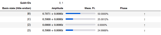
Note that the Q# code doesn’t have access to the output of DumpMachine, so you don’t need to resist the temptation to write any non-physical code, such as making decisions based on the amplitude of a certain basis state!
Similarly, DumpRegister allows you to print the quantum state of one part of the quantum system, as long as it’s not entangled with the rest of the system.
Finally, you can use %config magic command (available only in Q# Jupyter Notebooks) to tweak the format of DumpMachine output. It offers a lot of settings convenient in different scenarios. For example, by default DumpMachine uses little-endian integers to denote the basis states (the first column of the output); if you find raw bit strings easier to read, you can use %config dump.basisStateLabelingConvention="Bitstring" to switch.
Display the matrix implemented by the operation
Let’s say you’re working on a unitary synthesis task, implementing a quantum gate described by a matrix. You’ve written a Q# operation and want to check that it implements exactly the unitary matrix you’re looking for.
The DumpOperation library operation offers you a short and elegant way to do this. It takes an operation that acts on an array of qubits as a parameter (if your operation acts on a single qubit, like most intrinsic gates, or on a mix of individual qubits and qubit arrays, you’ll need to write a wrapper for it to use DumpOperation on it), and prints a matrix implemented by this operation. For example, DumpOperation(2, ApplyToFirstTwoQubitsCA(CNOT, _)); will print the matrix of the CNOT gate.

Note that this matrix might differ from the one you are used to seeing in quantum computing resources. DumpOperation uses the little-endian encoding for converting basis states to the indices of matrix elements. Thus, the second column of the CNOT matrix corresponds to the input state |1⟩ LE = |10⟩, which the CNOT gate converts to |11⟩ = |3⟩LE, meaning that the last element of this column is going to be 1, and the rest of the elements will be 0s.
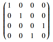
On the other hand, a lot of resources on quantum computing use big-endian encoding, in which the second column of the CNOT matrix corresponds to the input state |1⟩BE = |01⟩, which should be left unchanged by the CNOT gate, meaning that the 2nd element of this column will be 1, and the rest of the elements will be 0s. This convention will produce the familiar CNOT matrix:
Display the circuit performed by the operation
Quantum circuits are a very common way of visualizing the execution of quantum programs; you’ll see them in a lot of tutorials, papers, and books on quantum computing. Quantum circuits are a less powerful way of expressing the quantum computation compared to a quantum program. They don’t offer a good way to show the values of classical variables and their evolution, the decisions made based on the classical parameters or the measurement results, or even flow control structures such as loops or conditional statements. At the same time, they can be convenient to get a quick idea of what the program did, or to compare your implementation to the one offered in a book as a circuit.
%trace magic command (available only in Q# Jupyter Notebooks) offers a way to trace one run of the Q# program and to build a circuit based on that execution. Note that these circuits include only the quantum gates executed by the program during one run. They might differ in different runs of the same program, if that program takes parameters, has conditional branching or other behaviors that can change the sequence of gates applied by the program.
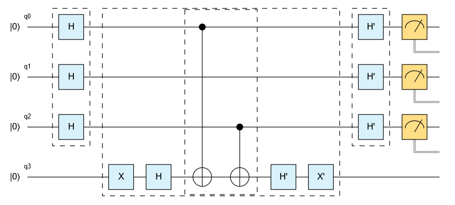
Here, for example, is the circuit printed using %trace for Q# program that implements Deutsch-Jozsa algorithm.

You see that initially the circuit focuses on high-level operations used in the root operation, showing them as blocks. The visualization is interactive, allowing you to click on each block to drill down to the intrinsic gates:
Run through the program execution while tracking the quantum state
The final tool in the list is the %debug magic command (available only in Q# Jupyter Notebooks) which allows you to combine tracing the program execution (as a circuit) and observing the program state as it evolves at the same time.
Here is a brief video of the %debug results for the same Deutsch-Jozsa algorithm operation for 2-qubit function. We switch to observing real and imaginary components of the amplitudes instead of measurement probabilities in the beginning of the program. For Deutsch-Jozsa algorithm, the probabilities of measuring each basis state during the program execution remain pretty much the same, it’s the signs of the amplitudes we want to watch for. For other algorithms, such as Grover’s search algorithm or quantum Fourier transform, observing measurement probabilities or the phases of the states can be more interesting.
Note that the %debug session requires the user to click through each of the steps and does not end until the program run is complete.
Conclusion
We hope you’ll find these tools useful in your work with the QDK, regardless of whether you are at the beginning of your quantum computing journey and seeking to confirm your understanding of the basics, or an experienced quantum software developer looking for that bug that’s been driving you crazy.
And if you want to practice using these tools and interpreting their output before using them for your work, check out our new VisualizationTools tutorial! As usual for the Quantum Katas tutorials, it offers detailed descriptions of the various tools listed here, demos, and hands-on exercises.
 Light
Light Dark
Dark
1 comment
Congrats Mariia and Team, looks pretty neat!