
Automate Resource Estimation with QIR
We have recently launched the new Azure Quantum Resource Estimator, which allows you to estimate the physical resources (number of physical qubits and wall clock runtime) required to run a quantum program on a fault-tolerant quantum computer. The fault-tolerant quantum computer is modeled using parameters that characterize the physical qubits and the quantum error correction scheme. The easiest way to get started is through the Azure Portal using an Azure Quantum Workspace. You will find many samples in the Sample Gallery’s Resource Estimation section.
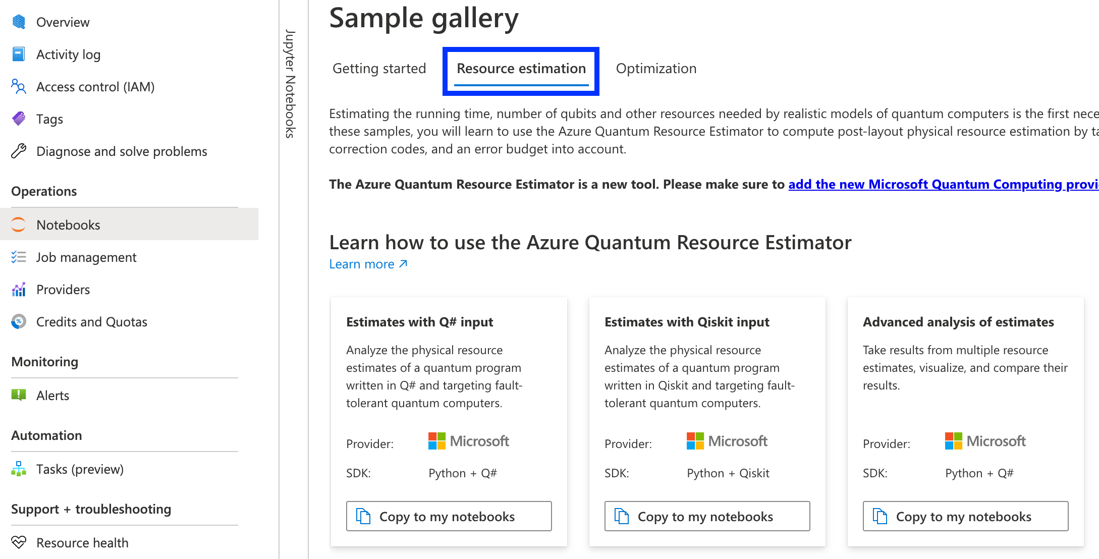
In these samples, e.g., Estimation with Q# input, you can generate resource estimations like the following that are computed from a quantum program that multiplies two quantum registers (click on the titles to unfold more tables with details on the estimates):
Physical resource estimates
| Physical qubits | 8160 |
Number of physical qubits This value represents the total number of physical qubits, which is the sum of 4200 physical qubits to implement the algorithm logic, and 3960 physical qubits to execute the T factories that are responsible to produce the T states that are consumed by the algorithm. |
| Runtime | 6ms 80us |
Total runtime This is a runtime estimate (in nanosecond precision) for the execution time of the algorithm. In general, the execution time corresponds to the duration of one logical cycle (10us) multiplied by the 608 logical cycles to run the algorithm. If however the duration of a single T factory (here: 82us 500ns) is larger than the algorithm runtime, we extend the number of logical cycles artificially in order to exceed the runtime of a single T factory. |
Resource estimates breakdown
| Logical algorithmic qubits | 84 |
Number of logical qubits for the algorithm after layout Laying out the logical qubits in the presence of nearest-neighbor constraints requires additional logical qubits. In particular, to layout the logical qubits in the input algorithm, we require in total logical qubits. |
| Algorithmic depth | 608 |
Number of logical cycles for the algorithm To execute the algorithm using Parallel Synthesis Sequential Pauli Computation (PSSPC), operations are scheduled in terms of multi-qubit Pauli measurements, for which assume an execution time of one logical cycle. Based on the input algorithm, we require one multi-qubit measurement for the 8 single-qubit measurements, the 0 arbitrary single-qubit rotations, and the 0 T gates, three multi-qubit measurements for each of the 192 CCZ and 8 CCiX gates in the input program, as well as No rotations in algorithm multi-qubit measurements for each of the 0 non-Clifford layers in which there is at least one single-qubit rotation with an arbitrary angle rotation. |
| Logical depth | 608 |
Number of logical cycles performed This number is usually equal to the logical depth of the algorithm, which is 608. However, in the case in which a single T factory is slower than the execution time of the algorithm, we adjust the logical cycle depth to exceed the T factory’s execution time. |
| Number of T states | 800 |
Number of T states consumed by the algorithm To execute the algorithm, we require one T state for each of the 0 T gates, four T states for each of the 192 CCZ and 8 CCiX gates, as well as No rotations in algorithm for each of the 0 single-qubit rotation gates with arbitrary angle rotation. |
| Number of T factories | 11 |
Number of T factories capable of producing the demanded 800 T states during the algorithm’s runtime The total number of T factories 11 that are executed in parallel is computed as |
| Number of T factory invocations | 73 |
Number of times all T factories are invoked In order to prepare the 800 T states, the 11 copies of the T factory are repeatedly invoked 73 times. |
| Physical algorithmic qubits | 4200 |
Number of physical qubits for the algorithm after layout The 4200 are the product of the 84 logical qubits after layout and the 50 physical qubits that encode a single logical qubit. |
| Physical T factory qubits | 3960 |
Number of physical qubits for the T factories Each T factory requires 360 physical qubits and we run 11 in parallel, therefore we need qubits. |
| Required logical qubit error rate | 9.79e-9 |
The minimum logical qubit error rate required to run the algorithm within the error budget The minimum logical qubit error rate is obtained by dividing the logical error probability 5.00e-4 by the product of 84 logical qubits and the total cycle count 608. |
| Required logical T state error rate | 6.25e-7 |
The minimum T state error rate required for distilled T states The minimum T state error rate is obtained by dividing the T distillation error probability 5.00e-4 by the total number of T states 800. |
| Number of T states per rotation | No rotations in algorithm |
Number of T states to implement a rotation with an arbitrary angle The number of T states to implement a rotation with an arbitrary angle is [arXiv:2203.10064]. For simplicity, we use this formula for all single-qubit arbitrary angle rotations, and do not distinguish between best, worst, and average cases. |
Logical qubit parameters
| QEC scheme | surface_code |
Name of QEC scheme You can load pre-defined QEC schemes by using the name |
| Code distance | 5 |
Required code distance for error correction The code distance is the smallest odd integer greater or equal to |
| Physical qubits | 50 |
Number of physical qubits per logical qubit The number of physical qubits per logical qubit are evaluated using the formula 2 * codeDistance * codeDistance that can be user-specified. |
| Logical cycle time | 10us |
Duration of a logical cycle in nanoseconds The runtime of one logical cycle in nanoseconds is evaluated using the formula 20 * oneQubitMeasurementTime * codeDistance that can be user-specified. |
| Logical qubit error rate | 2.37e-11 |
Logical qubit error rate The logical qubit error rate is computed as |
| Crossing prefactor | 0.08 |
Crossing prefactor used in QEC scheme The crossing prefactor is usually extracted numerically from simulations when fitting an exponential curve to model the relationship between logical and physical error rate. |
| Error correction threshold | 0.0015 |
Error correction threshold used in QEC scheme The error correction threshold is the physical error rate below which the error rate of the logical qubit is less than the error rate of the physical qubit that constitute it. This value is usually extracted numerically from simulations of the logical error rate. |
| Logical cycle time formula | 20 * oneQubitMeasurementTime * codeDistance |
QEC scheme formula used to compute logical cycle time This is the formula that is used to compute the logical cycle time 10us. |
| Physical qubits formula | 2 * codeDistance * codeDistance |
QEC scheme formula used to compute number of physical qubits per logical qubit This is the formula that is used to compute the number of physical qubits per logical qubits 50. |
T factory parameters
| Physical qubits | 360 |
Number of physical qubits for a single T factory This corresponds to the maximum number of physical qubits over all rounds of T distillation units in a T factory. A round of distillation contains of multiple copies of distillation units to achieve the required success probability of producing a T state with the expected logical T state error rate. |
| Runtime | 82us 500ns |
Runtime of a single T factory The runtime of a single T factory is the accumulated runtime of executing each round in a T factory. |
| Number of output T states per run | 1 |
Number of output T states produced in a single run of T factory The T factory takes as input 345 noisy physical T states with an error rate of 0.01 and produces 1 T states with an error rate of 2.52e-7. |
| Number of input T states per run | 345 |
Number of physical input T states consumed in a single run of a T factory This value includes the physical input T states of all copies of the distillation unit in the first round. |
| Distillation rounds | 2 |
The number of distillation rounds This is the number of distillation rounds. In each round one or multiple copies of some distillation unit is executed. |
| Distillation units per round | 23, 1 |
The number of units in each round of distillation This is the number of copies for the distillation units per round. |
| Distillation units | 15-to-1 space efficient physical, 15-to-1 space efficient logical |
The types of distillation units These are the types of distillation units that are executed in each round. The units can be either physical or logical, depending on what type of qubit they are operating. Space-efficient units require fewer qubits for the cost of longer runtime compared to Reed-Muller preparation units. |
| Distillation code distances | 1, 3 |
The code distance in each round of distillation This is the code distance used for the units in each round. If the code distance is 1, then the distillation unit operates on physical qubits instead of error-corrected logical qubits. |
| Number of physical qubits per round | 276, 360 |
The number of physical qubits used in each round of distillation The maximum number of physical qubits over all rounds is the number of physical qubits for the T factory, since qubits are reused by different rounds. |
| Runtime per round | 4us 500ns, 78us |
The runtime of each distillation round The runtime of the T factory is the sum of the runtimes in all rounds. |
| Logical T state error rate | 2.52e-7 |
Logical T state error rate This is the logical T state error rate achieved by the T factory which is equal or smaller than the required error rate 6.25e-7. |
Pre-layout logical resources
| Logical qubits (pre-layout) | 33 |
Number of logical qubits in the input quantum program We determine 84 from this number by assuming to align them in a 2D grid. Auxiliary qubits are added to allow for sufficient space to execute multi-qubit Pauli measurements on all or a subset of the logical qubits. |
| T gates | 0 |
Number of T gates in the input quantum program This includes all T gates and adjoint T gates, but not T gates used to implement rotation gates with arbitrary angle, CCZ gates, or CCiX gates. |
| Rotation gates | 0 |
Number of rotation gates in the input quantum program This is the number of all rotation gates. If an angle corresponds to a Pauli, Clifford, or T gate, it is not accounted for in this number. |
| Rotation depth | 0 |
Depth of rotation gates in the input quantum program This is the number of all non-Clifford layers that include at least one single-qubit rotation gate with an arbitrary angle. |
| CCZ gates | 192 |
Number of CCZ-gates in the input quantum program This is the number of CCZ gates. |
| CCiX gates | 8 |
Number of CCiX-gates in the input quantum program This is the number of CCiX gates, which applies controlled on two control qubits [1212.5069]. |
| Measurement operations | 8 |
Number of single qubit measurements in the input quantum program This is the number of single qubit measurements in Pauli basis that are used in the input program. Note that all measurements are counted, however, the measurement result is is determined randomly (with a fixed seed) to be 0 or 1 with a probability of 50%. |
Assumed error budget
| Total error budget | 1.00e-3 |
Total error budget for the algorithm The total error budget sets the overall allowed error for the algorithm, i.e., the number of times it is allowed to fail. Its value must be between 0 and 1 and the default value is 0.001, which corresponds to 0.1%, and means that the algorithm is allowed to fail once in 1000 executions. This parameter is highly application specific. For example, if one is running Shor’s algorithm for factoring integers, a large value for the error budget may be tolerated as one can check that the output are indeed the prime factors of the input. On the other hand, a much smaller error budget may be needed for an algorithm solving a problem with a solution which cannot be efficiently verified. This budget is uniformly distributed and applies to errors to implement logical qubits, an error budget to produce T states through distillation, and an error budget to synthesize rotation gates with arbitrary angles. Note that for distillation and rotation synthesis, the respective error budgets and are uniformly distributed among all T states and all rotation gates, respectively. If there are no rotation gates in the input algorithm, the error budget is uniformly distributed to logical errors and T state errors. |
| Logical error probability | 5.00e-4 |
Probability of at least one logical error This is one third of the total error budget 1.00e-3 if the input algorithm contains rotation with gates with arbitrary angles, or one half of it, otherwise. |
| T distillation error probability | 5.00e-4 |
Probability of at least one faulty T distillation This is one third of the total error budget 1.00e-3 if the input algorithm contains rotation with gates with arbitrary angles, or one half of it, otherwise. |
| Rotation synthesis error probability | 0.00e0 |
Probability of at least one failed rotation synthesis This is one third of the total error budget 1.00e-3. |
Physical qubit parameters
| Qubit name | qubit_maj_ns_e6 |
Some descriptive name for the qubit model You can load pre-defined qubit parameters by using the names |
| Instruction set | Majorana |
Underlying qubit technology (gate-based or Majorana) When modeling the physical qubit abstractions, we distinguish between two different physical instruction sets that are used to operate the qubits. The physical instruction set can be either gate-based or Majorana. A gate-based instruction set provides single-qubit measurement, single-qubit gates (incl. T gates), and two-qubit gates. A Majorana instruction set provides a physical T gate, single-qubit measurement and two-qubit joint measurement operations. |
| Single-qubit measurement time | 100 ns |
Operation time for single-qubit measurement (t_meas) in ns This is the operation time in nanoseconds to perform a single-qubit measurement in the Pauli basis. |
| Two-qubit measurement time | 100 ns |
Operation time for two-qubit measurement in ns This is the operation time in nanoseconds to perform a non-destructive two-qubit joint Pauli measurement. |
| T gate time | 100 ns |
Operation time for a T gate This is the operation time in nanoseconds to execute a T gate. |
| Single-qubit measurement error rate | 1E-06 |
Error rate for single-qubit measurement This is the probability in which a single-qubit measurement in the Pauli basis may fail. |
| Two-qubit measurement error rate | 1E-06 |
Error rate for two-qubit measurement This is the probability in which a non-destructive two-qubit joint Pauli measurement may fail. |
| T gate error rate | 0.01 |
Error rate to prepare single-qubit T state or apply a T gate (p_T) This is the probability in which executing a single T gate may fail. |
Assumptions
-
More details on the following lists of assumptions can be found in the paper Accessing requirements for scaling quantum computers and their applications.
-
Uniform independent physical noise. We assume that the noise on physical qubits and physical qubit operations is the standard circuit noise model. In particular we assume error events at different space-time locations are independent and that error rates are uniform across the system in time and space.
-
Efficient classical computation. We assume that classical overhead (compilation, control, feedback, readout, decoding, etc.) does not dominate the overall cost of implementing the full quantum algorithm.
-
Extraction circuits for planar quantum ISA. We assume that stabilizer extraction circuits with similar depth and error correction performance to those for standard surface and Hastings-Haah code patches can be constructed to implement all operations of the planar quantum ISA (instruction set architecture).
-
Uniform independent logical noise. We assume that the error rate of a logical operation is approximately equal to its space-time volume (the number of tiles multiplied by the number of logical time steps) multiplied by the error rate of a logical qubit in a standard one-tile patch in one logical time step.
-
Negligible Clifford costs for synthesis. We assume that the space overhead for synthesis and space and time overhead for transport of magic states within magic state factories and to synthesis qubits are all negligible.
-
Smooth magic state consumption rate. We assume that the rate of T state consumption throughout the compiled algorithm is almost constant, or can be made almost constant without significantly increasing the number of logical time steps for the algorithm.
«We have found the Resource Estimator simple to use despite the complexity of fault-tolerant computing schemes. In this tool, resource estimates are neatly laid-out at a glance, and hardware parameters and model assumptions can be easily tweaked. This kind of tool represents exactly what will be needed for designing large-scale algorithms and computations that are more resource-efficient, which is a major focus of our work.», notes Jing Hao CHAI, Fault-tolerant Quantum Computing Scientist at Entropica Labs.
To use the Resource Estimator in your day-to-day quantum computing work, and especially to automate multiple resource estimation jobs, it may be more convenient to integrate it directly into your existing toolchains or workflows. In this blog post, we will we use the Azure Quantum Python library to write a Python tool that returns resource estimates in JSON format given as input a QIR program. The complete source code is available in this Gist.

With the tool it will be possible to generate physical resource estimates as simple as:
python estimate.py quantum_program.qir > resources.json
Building the tool
Let’s start by declaring some program arguments:
import argparse, os

parser = argparse.ArgumentParser(
    prog="estimate",
    description="Estimate physical resources using Azure Quantum")

parser.add_argument("filename", help="Quantum program (.ll, .qir, .bc)")
parser.add_argument("-r", "--resource-id",
    default=os.environ.get("AZURE_QUANTUM_RESOURCE_ID"),
    help="Resource ID of Azure Quantum workspace (must be set, unless set via \
          environment variable AZURE_QUANTUM_RESOURCE_ID)")
parser.add_argument("-l", "--location",
    default=os.environ.get("AZURE_QUANTUM_LOCATION)"),
    help="Location of Azure Quantum workspace (must be set, unless set via \
          environment AZURE_QUANTUM_LOCATION")
parser.add_argument("-p", "--job-params", help="JSON file with job parameters")

args = parser.parse_args()
The Python tool takes a QIR program as input, which can be either in human-readable LLVM code (.ll and .qir extension) or directly in bitcode (.bc extension). The tool also requires information on how to connect with your Azure Quantum workspace, which can be either passed as program arguments or using environment variables. An Azure Quantum workspace allows us to access the resource estimator target and submit resource estimation jobs. If you do not have an Azure account, you can set one up for free here. If you do not have an Azure Quantum workspace, create one here. You will find the resource id and the location in the Overview page of your Azure Quantum workspace.
Next, we are connecting to our Azure Quantum workspace:
from azure.quantum import Workspace

workspace = Workspace(resource_id=args.resource_id, location=args.location)
The QIR program can be generated from other quantum programming languages like Q# (more details on generating QIR from Q#) and Qiskit (more details on generating QIR from Qiskit). If the QIR is provided in human-readable LLVM code, we first need to translate it to LLVM bitcode via the PyQIR library:
from pyqir.generator import ir_to_bitcode

ext = os.path.splitext(args.filename)[1].lower()
if ext in ['.qir', '.ll']:
    with open(args.filename, 'r') as f:
        bitcode = ir_to_bitcode(f.read())
elif ext == '.bc':
    with open(args.filename, 'rb') as f:
        bitcode = f.read()
In addition to the quantum program, one can pass job parameters that model the assumed fault-tolerant quantum computer. If no job parameters are specified, a default model is assumed. You can find more information on the job parameters in the Azure Quantum documentation. Job parameters can be provided through an optional JSON file such as the following:
{
    "qubitParams": {"name": "qubit_maj_ns_e6"},
    "qecScheme": {"name": "floquet_code"},
    "errorBudget": 0.005
}
We read such a file using Python’s json library:
import json

input_params = {}
if args.job_params:
    with open(args.job_params, 'r') as f:
        input_params = json.load(f)
Now that we have access to the Azure Quantum workspace, the QIR program, and the job parameters, we are ready to create and submit a resource estimation job:
from azure.quantum import Job
job = Job.from_input_data(
    workspace=workspace,
    name="Estimation job",
    target="microsoft.estimator",
    input_data=bitcode,
    provider_id="microsoft-qc",
    input_data_format="qir.v1",
    output_data_format="microsoft.resource-estimates.v1",
    input_params=input_params
)
job.wait_until_completed()
Now all what is left to do is to extract the results from the job and print them in JSON format:
result = job.get_results()
print(json.dumps(result, indent=4))
The resulting output looks as follows:
{
    // ...
    "physicalCounts": {
        "breakdown": {
            "algorithmicLogicalDepth": 3479912,
            "algorithmicLogicalQubits": 217,
            "cliffordErrorRate": 0.001,
            "logicalDepth": 3479912,
            "numTfactories": 18,
            "numTfactoryRuns": 242135,
            "numTsPerRotation": 15,
            "numTstates": 4358430,
            "physicalQubitsForAlgorithm": 191394,
            "physicalQubitsForTfactories": 599760,
            "requiredLogicalQubitErrorRate": 4.4141872274122407e-13,
            "requiredLogicalTstateErrorRate": 7.648013925503755e-11
        },
        "physicalQubits": 791154,
        "runtime": 29231260800
    },
    // ...
}
Next steps
Here are some ideas on what to try next:
- Try out the resource estimation tool in the Azure Portal
- Modify the Python program to support Q# and Qiskit programs directly as input files
- Modify the Python program to print a resource estimation table to the terminal instead of JSON data
 Light
Light Dark
Dark
0 comments