Analyzing a Sudoku solver using resources estimation

Mariia Mykhailova

This post is part of the Q# Advent Calendar 2021. Check out the calendar for more great posts!

A couple of months ago one of our users asked a very interesting question about one of the projects in our samples repository. The gist of the question was: Grover’s search-based Sudoku solver worked fine for one input puzzle but threw an exception when switched to a different puzzle. What’s going on, and might it be a memory issue?

Right now, quantum software development is at a stage where this type of questions – trying to troubleshoot unfamiliar quantum code developed by someone else – are very rare for most people outside of teams working on quantum software daily. But, similarly to classical software, eventually the field will grow so that such questions will be routine. I figured out that it would be interesting to use this question to show some tricks that can be used to answer it without getting familiar with every line of code.

Quick refresher: this is a simulation!

In the past Q# Advent Calendars I wrote about solving constraint satisfaction problems using Grover’s search, some challenges arising in the process and some tricks to overcome them. In the latest post of the series I dealt with a related issue: the program ran successfully but took longer than I liked to complete.

Both the out-of-memory issue and the too-long-runtime issue can stem from the same cause: using too many qubits in a program that runs on a full state quantum simulator – a classical program which models the behavior of a quantum system without accessing actual quantum hardware. A full state simulator uses 2ᴺ complex numbers to describe the state of an N-qubit system, so the more qubits the program uses at once, the more memory its state representation takes, and the more time it takes to update the state of the system after each gate application.

The rule of thumb I use is that programs which use under 25 qubits run within a reasonable time and memory footprint, programs which use over 35 qubits do not, and programs between these two extremes can vary. Let’s see where this Sudoku solver program falls on this spectrum!

Find circuit width before running the sample

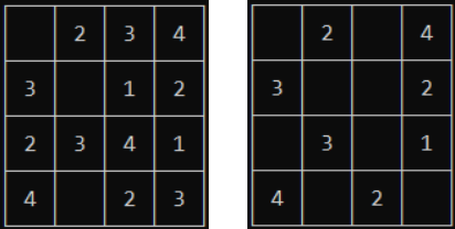
To start with, let’s minimize the classical portion of the code. I’m going to work with just 4×4 Sudoku puzzles, dropping digits from the grid as needed, so I’ll remove all code related to parsing command line parameters, working with other puzzle sizes, and the classical solution. I’ll start with the puzzle included in the sample (on the left) and see if I can work our way up to the puzzle suggested in the issue (on the right):

Next, let’s create QuantumSimulator inside the SudokuQuantum.QuantumSolve method instead of passing it as a parameter. I’m going to use the same two simulators each time I try to solve the puzzle, so it makes sense to create both inside the method.

The next step is to split the code inside SudokuQuantum.QuantumSolve method into three parts: parsing the input puzzle into a set of constraints that need to be satisfied, estimating the resources required for the quantum solution, and running the quantum solution. The basic code for resources estimation is very simple: you just need to create a separate simulator called ResourcesEstimator and pass it as the simulator parameter to the SolvePuzzle.Run method, extracting the necessary statistics afterwards:

var estimator = new ResourcesEstimator();
SolvePuzzle.Run(estimator, emptySquares.Count, size, 
    emptySquareEdgesQArray, startingNumberConstraintsQArray).Wait();
Console.WriteLine(estimator.Data.Rows.Find("QubitCount")["Sum"]);

However, at this point we hit a runtime exception ExecutionFailException that we didn’t see when running the Q# code on a full state simulator. Where does it come from?

Q# operation SolvePuzzle tries to solve the puzzle using different numbers of Grover iterations from 1 to the optimal number calculated with the assumption that there is exactly one solution to the provided puzzle. On each attempt the code checks whether the obtained result is correct, and if it is not, tries the next number of iterations, eventually giving up and throwing this exception to indicate that the solution was not found.

Resources estimator, however, does not actually simulate the gates applied by the code – it only goes through them, tracking events such as gates applications and qubit allocations. This allows this simulator to process programs that require hundreds and thousands of qubits, but on the flip side, whenever it encounters a measurement, it always assumes that the measurement result is 0, thus never realizing that the puzzle has a solution!

A more advanced resources estimator called QCTraceSimulator allows to provide probabilities of measurement outcomes to use in resources estimation, but this is out of scope of this blog post.

Once we rewrite SolvePuzzle to run the search just once and to remove the correctness check (it is repeated by the classical code afterwards anyways), we can see that this program is going to use 27 qubits, so it can be simulated. However, if we remove 5 more digits from the puzzle to get the input suggested in the original issue, the qubit count will jump to 81 – which is a lot more than can be simulated!

Diving deeper: where are the qubits used?

Why does such a small program use so many qubits? Let’s fall back to the original puzzle with 3 missing digits and see what we can figure out from reading the code.

On the surface, we need to find values for three variables (the numbers in the missing cells), each of which can range from 0 to 3, thus requiring 2 bits per variable – but this accounts only for 6 qubits. Where do 21 more come from?

• Checking answer correctness in Grover’s search (before refactoring to remove the check): 1 qubit. Operation FindColorsWithGrover allocates the qubit “output” used to verify the correctness of the answer alongside the register used for storing the variables, though it doesn’t use it until after the main iterations are done.
• Phase kickback trick: 1 qubit. Every time a Grover iteration applies the marking oracle that checks whether the variable assignment is a solution, it needs to convert it into a phase oracle using phase kickback trick, which uses an extra qubit.
• Constraints on the variables that cannot be equal: 2 qubits. Every time two missing digits are in the same row, column, or 2×2 square of the Sudoku grid, they add an inequality constraint on the matching variables, which needs a qubit to track it. In our cases two of the missing digits are in the top left square of the Sudoku grid, and two are in the second column, so there are two constraints.
• Constraints on the values the variables cannot take: 9 qubits. Similarly, for every missing digit every digit that is in the same row, column, or 2×2 square adds an inequality constraint, since the missing digit cannot take the same value as any of them. The classical part of the code does the pre-processing to remove duplicate constraints, but each constraint is checked using a separate qubit, so with each of the 3 variables having 3 values they cannot take, we need 9 qubits to track these constraints.
• If you look through the rest of the Q# code, you won’t find any more explicit qubit allocations, so where are the remaining 9 qubits coming from? Those are a sort of “virtual” qubits – qubits that you didn’t allocate explicitly, but that would have to be allocated by the compiler when running the code on hardware to implement the multi-controlled gates used in the ApplyVertexColoringOracle. Resources estimations target hardware execution, so they count those qubits even though they won’t be used when running on a simulator. The simulator only ever allocates 18 qubits, making the simulation comfortably within its simulation capabilities.

Optimizing the code

Can we optimize the code to be able to solve more complicated instances of the Sudoku puzzle?

The first and obvious optimization is changing the way to evaluate the constraints on the values that the variables cannot take. We can use one qubit per missing digit and evaluate all constraints that involve this digit using it. This allows us to save several qubits (6 for the small puzzle we follow in this blog post), but not enough to allow us to solve larger puzzles.

A better way is to rewrite Grover’s search implementation to build these checks in the search space rather than evaluate them as constraints on the variables. As a reminder, Grover’s search uses an equal superposition of all basis states in the search space both as its starting state and as a part of “reflection about the mean” step. We can use a superposition of only the states that satisfy the constraints imposed by existing digits in the grid. Not only does this reduce the number of constraints to check (and thus the number of qubits allocated), but it also reduces the number of iterations the search needs to do!

The details of this refactoring are out of scope for this blog post, but you can see the complete code here. You see that it can solve many puzzles without any search iterations – with enough digits the search space size is 1, and the correct answer is obtained by just preparing the “superposition” of one basis state and measuring it (this means that the solution is effectively classical, with all the work done by the preprocessing routines). And finally, it solves the puzzle mentioned in the issue with 8 missing digits correctly in just 2 search iterations, taking about 5 minutes!

Mariia Mykhailova Principal Software Engineer, Advanced Quantum Development

Follow