
What’s the deal with humongous objects in Java?
As a Software Engineer in Microsoft’s Java Engineering Group, part of my job is to analyze and improve the performance of Java’s garbage collectors. As a Java application runs, the garbage collector is responsible for allocating objects on the heap and freeing up heap space when those objects are no longer live. In this blog post, I’ll focus specifically on how the GC handles different volumes of live data and objects of various sizes.
If you’re running JDK 11 or later (and you should be), the default garbage collector is the Garbage First Garbage Collector (G1 GC). G1 is a regionalized collector, meaning that the Java heap is partitioned into a number of equal-sized regions. Regions sizes are a power of two and can range from 1 MB to 32 MB, sized such that there are at most 2048 regions. These regions are logically grouped into Eden, Survivor, and Tenured. Empty regions are considered Free and can become any of the other three. As G1 is a generational collector, new objects are allocated into Eden regions. Objects that have survived at least one GC cycle get copied into Survivor regions, and once those objects survive enough GC cycles, they are promoted to Tenured regions. One notable exception is humongous objects, which are allocated into contiguous Free regions instead of Eden. These regions become Humongous regions and are considered part of Tenured space.
What are humongous objects?
G1 considers all objects bigger than one-half of a memory region to be humongous objects. From JEP 278, humongous objects always take up a whole number of regions. If a humongous object is smaller than one region, then it takes up the whole region. If a humongous object is larger than N regions and smaller than (N+1) regions, then it takes up (N+1) regions. No allocations are allowed in the free space, if any, of the last region. Humongous objects can never be moved from one region to another.
What does this mean for the Java heap?
If humongous objects always take up a whole number of regions, certain sizes of humongous objects are more space efficient than others. Let’s take a look at an example heap with 32 MB regions. If regions are 32 MB, all objects over 16 MB are considered humongous.

Humongous objects that are slightly above the humongous threshold (in this example, just over 16 MB) or slightly greater than the size of N regions (just over 32 MB, 64 MB, etc.) result in significant space left over in humongous regions.
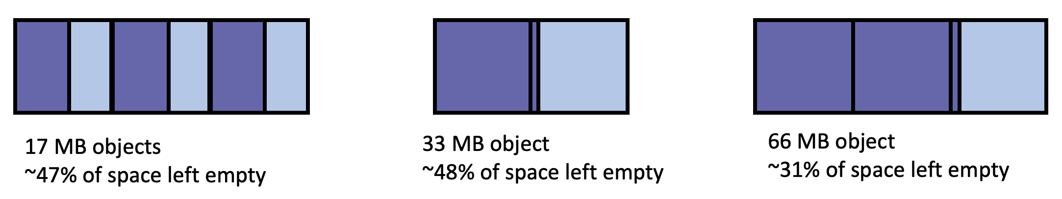
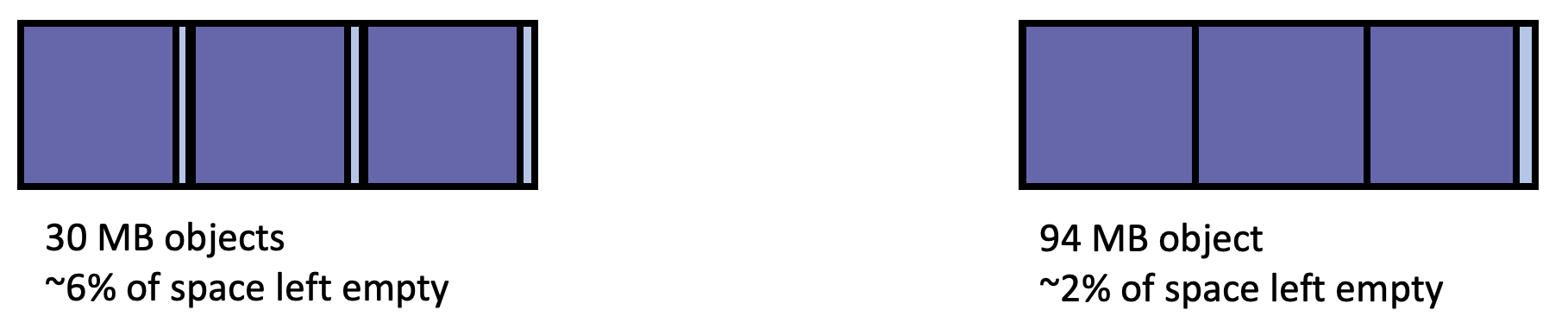
On the contrary, humongous objects that are slightly smaller than the size of N regions (just under 32 MB, 64 MB, etc.) occupy most of those regions with less empty space left over.
What does this mean for my application?
Based on the sizes of the allocated objects, the same volume of live data can actually take up different amounts of heap space. Let’s examine a few different scenarios and see how the GC responds.
I initially ran these benchmarks as part of a GC investigation with @Ana Marsh that didn’t focus specifically on humongous objects. Because of this, the following examples show the effect humongous objects can have on the heap in a real-world (albeit benchmarking) scenario.
In the first simulated system, long-lived data occupies 50% of the heap. In the second, long-lived data occupies 50% of the heap and medium-lived data occupies an additional 25% of the heap. For each system type, we tested how the GC performs both with and without humongous objects.
Running the Benchmark
We used the HyperAlloc benchmark developed by the Amazon Corretto team. HyperAlloc continuously allocates objects to achieve a target allocation rate and heap occupancy. Each newly allocated object is a random size between the specified minimum and maximum object sizes. I used Microsoft’s build of OpenJDK 17.0.2 with an 80 GB heap. For an 80 GB heap, heap regions are 32 MB by default, so all objects larger than 16 MB are treated as humongous. I tested the following combinations using CBL-Mariner Linux (version 2.0.20220226) on an Intel Xeon Silver 4210 Processor with 40 vCPUs (2 sockets, 10 cores per socket, 2 threads per core) and 376 GB of RAM:
- 50% of the heap is live with objects from 128 bytes – 16 MB
- 50% of the heap is live with objects from 128 bytes – 20 MB (humongous objects)
- 75% of the heap is live with objects from 128 bytes – 16 MB
- 75% of the heap is live with objects from 128 bytes – 20 MB (humongous objects)
If you’d like to follow along at home, here’s an example command line:
jdk-17.0.2+8/bin/java -Xms80G -Xmx80G -Xlog:gc*,gc+ref=debug,gc+phases=debug,gc+age=trace,safepoint:file=<GC log file> -XX:+AlwaysPreTouch -XX:+UseLargePages -XX:+UseTransparentHugePages -XX:ParallelGCThreads=40 -XX:+UseG1GC -javaagent:<jHiccup directory>/jHiccup.jar=-a -d 0 -i 1000 -l <jHiccup log file> -jar <HyperAlloc directory>/HyperAlloc-1.0.jar -a 4096 -h 81920 -s 40960 -d 600 -c false -t 40 -n 128 -x 655360 -l <CSV output file>
Let’s break this down a little:
| jdk-17.0.2+8/bin/java | path to the java executable we’re testing |
| -Xms80G -Xmx80G | set the initial and maximum heap size to 80 GB |
| -a 4096 | set the target allocation rate to 4 GB/s |
| -h 81920 | tell the benchmark the heap size is 80 GB |
| -s 40960 | set the target long-lived heap occupancy to 40 GB (50% of the heap) |
| -m 20480 | set the target mid-aged heap occupancy to 20 GB (25% of the heap) |
| -d 600 | set the benchmark duration to 600 seconds |
| -c false | set compressedOops support to false, needed for a 32 GB or larger heap |
| -t 40 | set the number of worker threads to 40 |
| -n 128 | set the minimum object size to 128 bytes |
| -x 16777216 | set the maximum object size to 16 MB |
I used 40 worker threads because my test machine has 40 vCPUs. For this investigation, a benchmark duration of 600 seconds is long enough to give us the necessary information. I used a target allocation rate of 4 GB/s, but in these four benchmark runs, my observed allocation rates ranged from 19 GB/s to 50 GB/s. The actual allocation rate depends on the number of worker threads and the size of allocated objects, so it may differ significantly from the target passed to HyperAlloc. This variation in the actual allocation rate isn’t an issue for us, but it’s something to be aware of if you’re trying to replicate this experiment.
I also used a few other JVM flags for these benchmarking runs. -XX:+AlwaysPreTouch tells the JVM to touch all bytes of the max heap size with a ‘0’, causing the heap to be allocated in physical memory instead of only in virtual memory. This reduces page access time as the application runs, as pages are already loaded into memory, but comes at the cost of increased JVM startup time. It’s often a good idea to enable pre-touch on large heaps or to simulate a long-running system. In Linux, we can increase the size of these pages using -XX:+UseLargePages and -XX:+UseTransparentHugePages. Aleksey Shipilëv’s blog post provides more information about the use cases and tradeoffs of using these flags.
The data in the following sections was collected using the following JVM logging options: -Xlog:gc*,gc+ref=debug,gc+phases=debug,gc+age=trace,safepoint. This blog post provides a good intro on Unified JVM Logging (JEP 158).
More information on how to set up and run the benchmark is available from the source at HyperAlloc’s README. To parse the generated GC logs, I used the open-source Microsoft GCToolkit.
Results
Now that we’ve run the benchmark, let’s look at the heap before and after GC. 50% of the heap is live and objects range from 128 bytes – 16 MB, so there are no humongous objects.
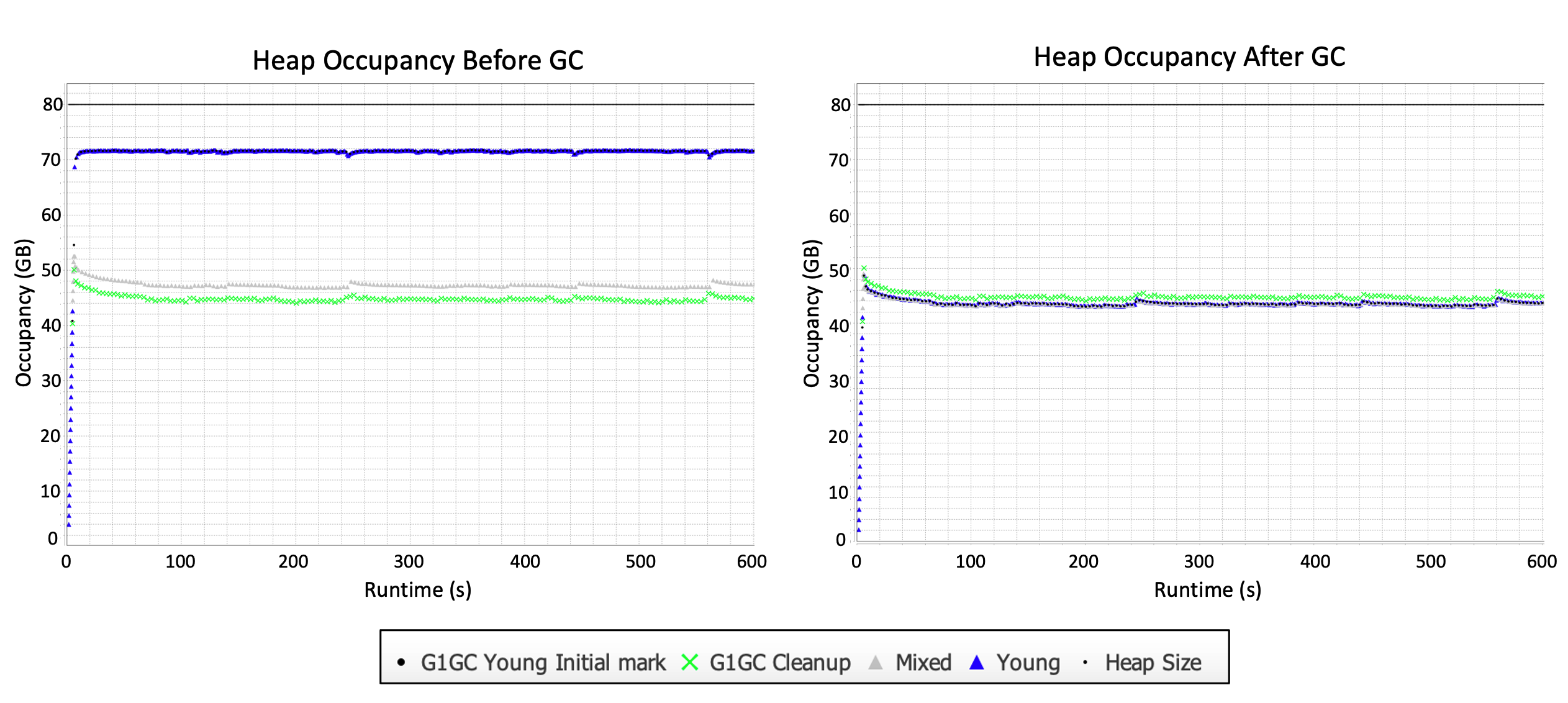
Each point on the graph on the left represents the heap occupancy at the instant before a GC event. The corresponding point at the same timestamp on the right shows the heap occupancy directly after that same GC event. Points are colored by the type of GC event (G1GC young initial mark, G1GC cleanup, mixed GC, and young GC). The most important thing to focus on here is the young GCs (shown as blue triangles).
The heap occupancy gets up to roughly 72 GB before a young GC is triggered. After a young GC, the heap occupancy is reduced to about 44 GB. We would expect this reduction because 50% of the heap (40 GB) is live for our simulated workload. The heap occupancy is 44 GB instead of 40 GB post-GC due to floating garbage after young GC (there are some objects that are no longer live that have not yet been collected). It’s worth noting that although this workload without humongous objects is our “least-stressed” scenario, we’re still allocating lots of data and putting plenty of pressure on the GC.
Now let’s see what the heap looks like when we add humongous objects. Here, 50% of the heap is live and objects range from 128 bytes – 20 MB:
In this case, the GC is a bit more stressed – the heap occupancy sometimes gets up to 78 GB before young GC! Another notable difference between this scenario and the previous one is the heap occupancy AFTER young GC. Now that we’ve added humongous objects, we see a post-GC heap occupancy of about 54 GB compared to the previous 44 GB. This time, the difference between the observed heap occupancy and the actual volume of live data is due to humongous objects.
In this scenario, 20% of the allocated objects are humongous objects, and these humongous objects make up 36% of the data volume. This means that of the 40 GB of live data, 25.6 GB lives in regular objects and 14.4 GB lives in humongous objects. The average humongous object in this workload is 18 MB. Because our region size is 32 MB, humongous regions are only 56.25% full on average. The 14.4 GB of data in humongous objects therefore occupies 25.6 GB of heap space, with 11.2 GB of unusable space trapped in humongous regions. We should expect to observe a heap occupancy of 51.2 GB (25.6 GB taken up by regular objects + 25.6 GB taken up by humongous objects). The additional difference between the projected 51.2 GB and the observed 54 GB is due floating garbage left after young GC.
The heap pressure due to humongous objects becomes even more prominent as the volume of live data increases. In the next example, 75% of the heap is live and objects range from 128 bytes – 16 MB (no humongous objects).
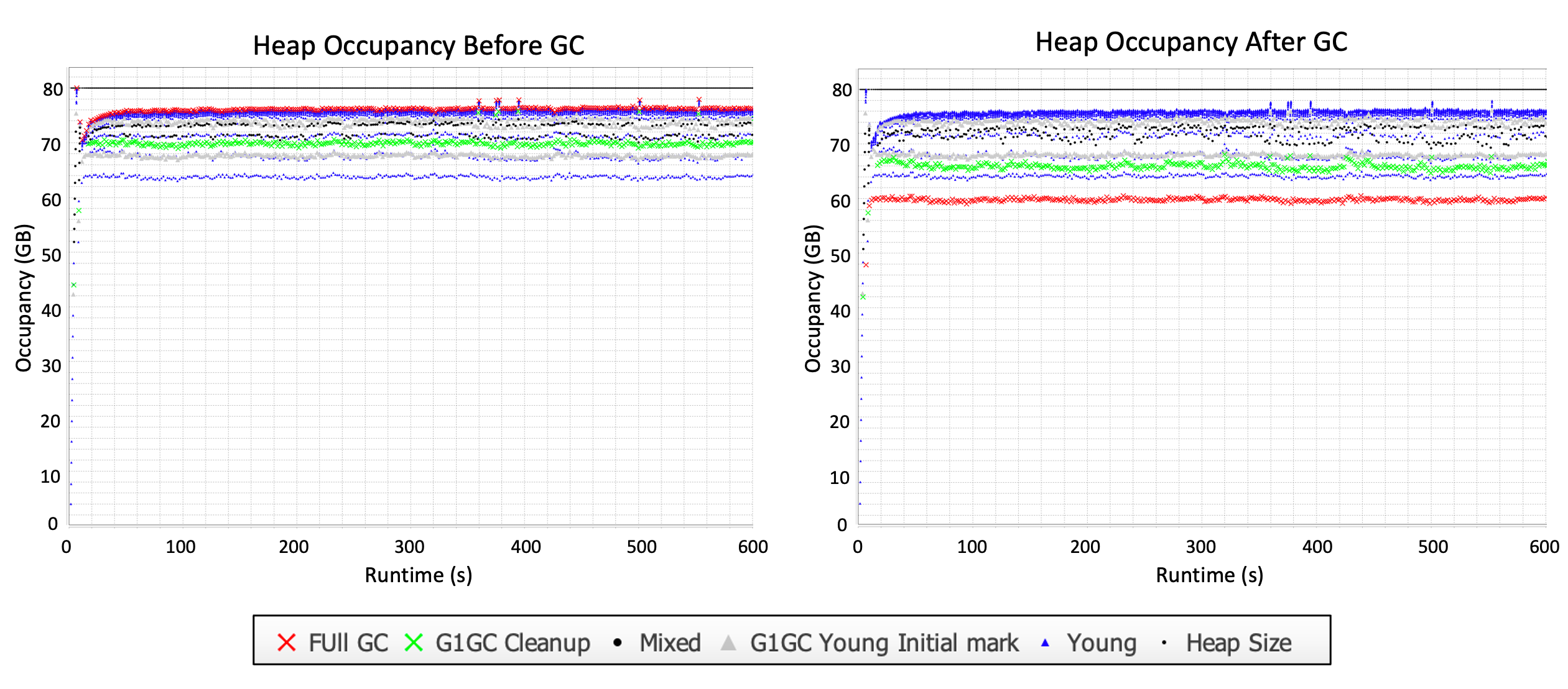
We’re really pushing the limits of G1 here. Now that 75% (60 GB) of the heap is live, we have less free space to accommodate transient data. Young GCs are first triggered when the heap occupancy reaches about 64 GB, but they cannot free up any space, as shown by nearly identical lines of points at 64 GB before and after young GC. Young GCs get triggered again when the heap occupancy rises to roughly 68 GB, 72 GB, and then 75 GB before going into a full GC. All garbage is collected during a full GC, reducing the heap occupancy to the expected 60 GB.
This is what the heap looks like when we add humongous objects. 75% of the heap is live and objects range from 128 bytes – 20 MB:
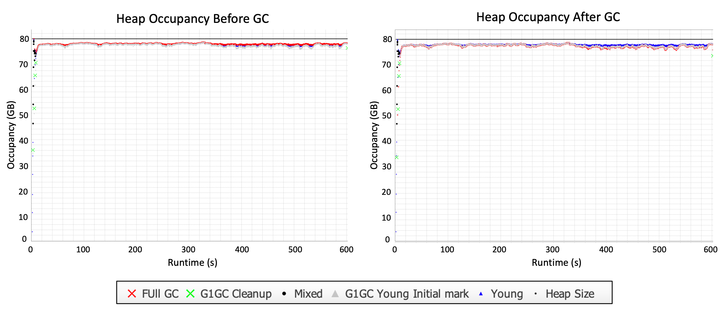
Wow. G1 is stressed and it SHOWS. Like in the previous case, young GCs don’t seem to be effective in reducing heap occupancy. However, unlike the previous case, the heap occupancy hovers at around 77 GB even after full GC.
Like in the second scenario, humongous objects make up 36% of the data volume. This means that of the 60 GB of live data, 38.4 GB lives in regular objects and 21.6 GB lives in humongous objects. Because the average humongous object is 18 MB, humongous regions are only 56.25% full on average. The 21.6 GB of data in humongous objects therefore occupies 38.4 GB of heap space, with 16.8 GB of unusable space trapped in humongous regions. We should expect to observe a heap occupancy of 76.8 GB (38.4 GB taken up by regular objects + 38.4 GB taken up by humongous objects). As a reminder, only 60 GB of our heap is supposed to be live – but because of humongous objects, we need roughly 77 GB to accommodate all the live data. This leaves very little space for transient data, resulting in near-constant GCs and significantly reduced throughput.
Testing the extremes
We came dangerously close to running out of heap space in the previous example – so what happens when we push G1 even further? To test this, I ran HyperAlloc again using workloads exclusively made up of humongous objects. I used an 80 GB heap with 32 MB regions, so all objects larger than 16 MB are treated as humongous:
- 75% of the heap is live with objects from 30 MB – 32 MB
- 75% of the heap is live with objects from 16 MB – 18 MB
In the first workload, humongous regions are 96.88% full on average. The 60 GB of data in humongous objects therefore occupies 61.9 GB of heap space, with only 1.9 GB of unusable space trapped in humongous regions. Even though all objects are humongous, there is enough heap space for the application to run smoothly.
In the second workload, humongous regions are only 53.13% full on average. The 60 GB of data in humongous objects therefore requires 112.94 GB of heap space – far more than our 80 GB heap! When I tested this, the benchmark crashed with an OutOfMemoryError in about 5 seconds.
What can I do?
If you notice that your application has higher-than-expected heap usage, you may have the same problem. If possible, it may be helpful to change the sizes of allocated objects to avoid humongous objects that result in wasted heap space. It may also be helpful to adjust the size of heap regions using -XX:G1HeapRegionSize= such that the problematic objects are no longer humongous, or experiment with using a different GC.
 Light
Light Dark
Dark
0 comments