Managing big cities and providing citizens public services requires municipalities to have a keen understanding of what citizens care the most about. And, as the cities we live in seek more and more to become the ‘smart cities’ of tomorrow, this means gathering and analyzing vast amounts of data. Data gathered from social and municipal sources enable municipalities to understand what specific trending issues citizens currently care most about, and to better understand how they feel about any given matter.

In this code story we’ll look at Commercial Software Engineering’s (CSE) recent collaboration with ZenCity, a startup focused on providing municipalities with insights gained through social and operational data. ZenCity’s platform provides municipalities with insights into topics currently discussed on social media and operational systems – from current security issues to upcoming events or festivals – the sentiment being expressed on each issue, and additional context such as specific locations related to issues. In engaging with Microsoft, ZenCity was interested in two outcomes: first, in expanding their offering with a detector for temporal patterns (i.e., points in time in which specific events pop up from the data) and second, in extending their data ingestion pipeline to better handle data at scale and new types of data.

Introducing temporal patterns into ZenCity’s system is an important addition to the product, as it allows the municipality to automatically detect urgent issues and can provide more contextual understanding of events. For example, such a module would enable the city to easily identify issues pertaining to a certain festival, a specific hazard, or any other event that occurred in the city.

Working with Zencity, we developed a system capable of detecting trending topics that is comprised of a data ingestion and preparation pipeline and a set of models capable of detecting interesting anomalies or trends. Additionally, we developed a supporting Spark-based pipeline capable of handling events gathered from various sources. In this code story we’ll focus on the data understanding and modeling part, and as an example we’ll use the San Francisco 311 data, available in the San Francisco Open Data portal.

Challenges and Solution

Detecting trending topics requires the processing of multiple textual items, often at scale, extracting one or more topics from each item, and then looking at the temporal characteristics of each topic and the entire set of topics. Our solution uses time series analysis methods for how much a topic is trending, as well as a pipeline for handling textual items from ingestion through text analytics to a statistical model that detects which topics are currently trending.

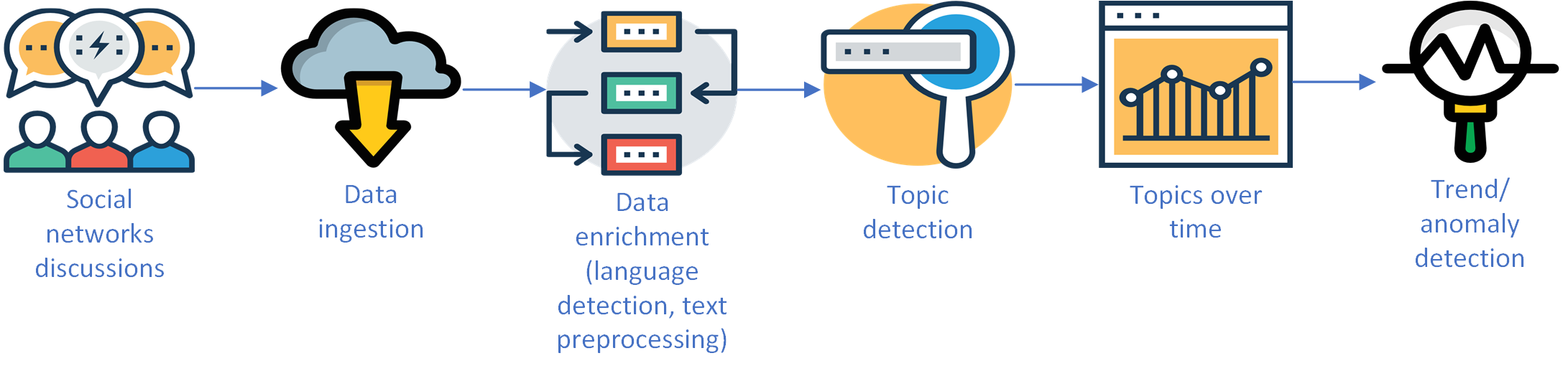
Figure 1 describes the data flow from a social network to a trending topics detection mechanism. Data from social networks or other sources is collected and ingested into the system. Then, various processes cleanse the data and enrich it (for example by detecting language or entities). For each item, a topic or multiple topics are extracted if found, and the count of items per topic over time is stored. The counts over time form a time series which can be analyzed for trends or anomalies.

 

 

Problem formulation

Trending topic detection is the ability to automatically extract topics which are temporally common than usual. Once topics are extracted for each body of text (e.g. tweets, Facebook posts or incidents on the city’s CRM – Customer-Relationship Management System), one can count the number of texts per topic over a fixed period of time (e.g. 1 hour), and look for differences between time windows. Changes of quantity between time windows can be caused by an external factor for a specific topic (e.g. a festival that took place in a city), an external factor for all topics altogether (e.g. citizens opened a new Facebook group), or a system internal factor, such as a change to the way topics are extracted or how texts are gathered from sources. It is important to distinguish the different cases, since in most cases only an external factor for a specific topic is of interest.

There are different types of patterns we can consider as a trend in a specific topic. Figure 2 shows three examples of such patterns.

 

 

Data understanding

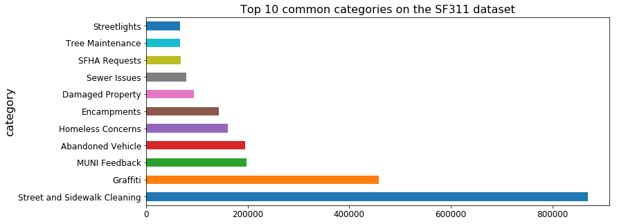
The San Francisco 311 Cases data holds ~3M records from calls to the 311 call-center from July 2008. Each record has a predefined category (topic). There are 102 categories on the dataset, some of which were only used for a certain period of the time. Out of the 102 categories, 46 have more than 1000 incidents and were used for more than 100 days. In this dataset, topics (categories) are predefined. When working with social network data, we used ZenCity’s proprietary topic extraction module.

Figure 3 shows the number of events per category for the top 10 most common categories.

 

 

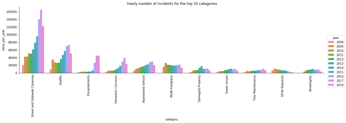
Different categories are used in different periods of time. Figure 4 shows the number of yearly incidents per category, for the top 10 categories. Some categories exhibit a trend from year to year, while others have relatively the same number of incidents per year.

 

In order to transform a set of incidents into intervals for time-series analysis and analyze trending topics, we developed moda, a python package for transforming and modeling such data. We’ll look more at moda in the experimentation section. Figure 5 shows the time series of one category, using 3 different time interval values. The following code snippet demonstrates how to turn the SF311 dataset into a time series that can be analyzed using moda:

import pandas as pd
from moda.dataprep import raw_to_ts, ts_to_range

DATAPATH = "SF-311_simplified.csv"
TIME_RANGE = "3H" # Aggregate into 3 hour intervals

# Read raw file
raw = pd.read_csv(DATAPATH)

# Turn the raw data into a time series (with date as a pandas DatetimeIndex)
ts = raw_to_ts(raw)

# Aggregate items per time and category, given a time interval
ranged_ts = ts_to_range(ts,time_range=TIME_RANGE)

For a full example, see this jupyter notebook.

Data preparation

The data preparation steps we used were the following:

1. Decide on a time interval, based on the business requirement and frequency of incidents. There is a trade-off between detecting changes quickly and the detection accuracy. We used a 24-hour window for small cities and 1-hour windows for bigger cities like San Francisco.
2. Count the number of incidents per time interval and handle additional information such as the number of shares/likes/retweets a post received.
3. Remove rare categories: If rare categories are also of less interest to the municipality, they can be removed by putting a lower bound to incident/post count.
4. Remove old categories: Some categories appear in the data but aren’t used by the municipality any longer.
5. Missing values handling: There are cases when a topic had no incidents on a specific time interval. We padded the time series with zero on such time intervals, as this is the real time series value at these points in time.
6. Decide on history size: In most cases, the entire history is unnecessary. We decided to look back 30 or 60 days. This constant might change for other datasets.

Approaches to modeling

As mentioned earlier, we focused on time series methods for modeling. Specifically, we looked at methods capable of identifying pulses, as it is the most frequent form of change that we have seen in the data. To find an optimal model, we evaluated different time series methods. Additional methods exist such as the ones surveyed in [1].

Moving average based seasonality decomposition (MA adapted for trendiness detection)

This method is a naive decomposition that uses a moving average to remove the trend, and a convolution filter to detect seasonality. The result is a time series of residuals. See [2] for additional information on seasonal decomposition. To detect anomalies and interesting trends in the time series, we look for outliers on the decomposed trend series and the residuals series. Points are considered outliers if their value is higher than a number of standard deviations of historical values. We evaluated different policies for trendiness prediction: residual anomaly only; trend anomaly only; residual OR trend anomaly; and residual AND trend anomaly.

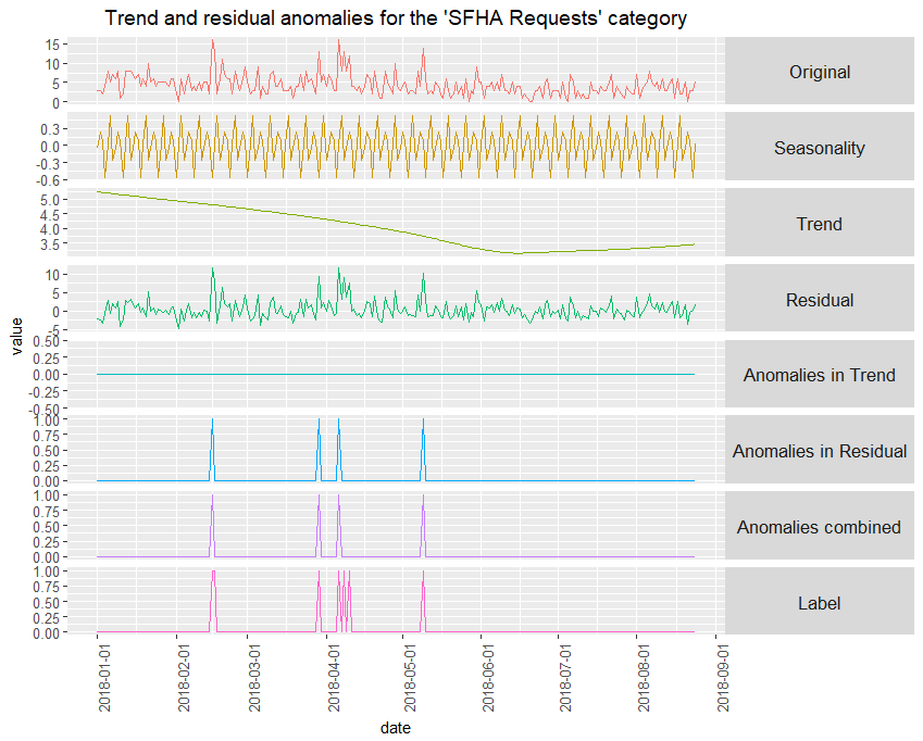
Seasonality and trend decomposition using Loess (Adapted STL)

STL uses iterative Loess smoothing [5] to obtain an estimate of the trend and then Loess smoothing again to extract a changing additive seasonal component. It can handle any type of seasonality, and the seasonality value can change over time. We used the same anomaly detection mechanism as the moving-average based seasonal decomposition. For more on this method see [2] and [4]. Figure 6 provides an example of running STL on one category, and how anomalies are calculated following the time series decomposition.

 

Azure Machine Learning Anomaly Detection API

Another way to look at the problem is strictly as an anomaly detection problem. The exploratory data analysis showed that most of the interesting areas are actually anomalies, in contrast to a large upward trend or a change point. We used the Azure Machine Learning Anomaly Detection API as a black box for detecting anomalies. We further used the upper bound of the time series provided by the tool to estimate the degree of anomaly.

Twitter Anomaly Detection

An anomaly detection method, which employs methods similar to STL and MA is the Twitter Anomaly Detection package. An initial experimentation showed good results, so we included it in the analysis. The official implementation is in R, and we used a 3rd party Python implementation which works a bit differently.

Univariate representation vs. multi-category representation

Anomalous patterns can appear for multiple topics at once. Some trending topics detection methods, such as the one proposed by Kostas Tsioutsiouliklis [3], represent the data as multi-category, and attempt to find topics that have a higher proportion than usual, in contrast to a higher quantity than usual. The pros of this method are that topics are always compared to others, and an increase in one topic only would be detected, while an increase in multiple topics should not change the topics distribution. In this analysis we model the problem while assuming independence among topics. It is possible to look for co-occurring trending topics as a post process.

Evaluation

Labeling

Four different time series datasets were manually labeled using the TagAnomaly labeling tool, which was built as a part of this engagement. TagAnomaly allows the labeler to view each category independently or jointly with other categories, to better understand the nature of the anomaly / shift. It further allows the labeler to look at the raw data in a specific time range, to see what the nature of the posts / incidents was about.

It is important to note that manual labels are highly subjective. For example, a weekly pattern for the topic “religion” could be interesting for some municipalities but irrelevant for others. Peaks in garbage collection could be interesting in some cases but could also be random outliers. In addition, some labelers are more conservative than others and would mark less points as interesting.

Metric

We evaluated each model by comparing the predicted trending timestamps with the timestamps labeled manually as trending. For short time intervals, or for trends spanning multiple timestamps, it is possible that the predicted and actual point in time are not completely aligned. Therefore, we implemented a soft evaluation metric, which looks for matches in a nearby window. For this method, the lookup window size is customizable. Then, we counted True Positives, False Positives and False Negatives from each category. These were used to calculate precision, recall, f1 and f0.5 for each category individually and for the entire dataset. Figure 7 shows the way metrics are calculated for this multi-category time series.

Figure 7: Metrics for multi-category classification used in this analysis

Experimentation

All models and evaluation code exist in moda. The package provides an interface for evaluating models on either univariate or multi-category datasets. It further allows the user to add additional models using a scikit-learn style API. All models described here were adapted to a multi-category scenario using the package’s abstract trend_detector class, which allows a univariate model to run on multiple categories. It further provides functionality for the evaluation of models using either a train/test split or a time-series cross validation. We also provide sample code for a grid-search hyper parameter optimization for different models.

The following code snippet shows how to run one model using moda:

from moda.evaluators import get_metrics_for_all_categories, get_final_metrics
from moda.dataprep import read_data
from moda.models import STLTrendinessDetector

model = STLTrendinessDetector(freq='24H', 
                              min_value=10,
                              anomaly_type='residual',
                              num_of_std=3, lo_delta=0)

# Take the entire time series and evaluate anomalies on all of it or just the last window(s)
prediction = model.predict(dataset)
raw_metrics = get_metrics_for_all_categories(dataset[['value']], prediction[['prediction']], dataset[['label']],
                                             window_size_for_metrics=1)
metrics = get_final_metrics(raw_metrics)

## Plot results for each category
model.plot(labels=dataset['label'])

Results

We compared the moving average seasonal decomposition, STL, Twitter’s model and Azure anomaly detector on four datasets: San Francisco 311 with 1H interval (SF 1H), San Francisco 311 with 24H interval (SF 24H), social network data for the city of Corona (Corona 12H), and social network data for the city of Pompano Beach (Pompano 24H). Here are the F1 scores:

	Adapted Moving Average Seasonal Decomposition	Adapted STL	Twitter Anomaly Detection	Azure Anomaly finder	Number of items	Number of categories	Number of samples
Corona 12H	0.68	0.7	0.74	0.73	21,800	37	2982
Pompano 24H	0.72	0.71	0.76	0.76	24,245	39	3308
SF 24H	0.69	0.75	0.57	0.38	385K	84	180K
SF 1H	0.35	0.31	0.28	0.09	385K	84	432K

Table 1: Results for 4 different datasets and 4 different models, and additional information on each dataset.

The entire run history with parameters values per run can be found here: https://www.comet.ml/omri374/trending-topics.

Conclusion

We can see that for datasets with 12/24 hour intervals, we get decent results. For a 1H interval dataset, F1 measure drops to 35%. There are two main reasons:

• The time series is much more volatile and sparser, thus harder to model
• There are more points in this dataset (432K vs 180K), so manual labeling is more difficult and more subjective

Figure 8 shows an example of the time series, the prediction (of adapted STL) and the manually labeled data for one category on the 1H dataset. The two reasons are apparent in this example. In most cases, the recall was higher than precision, so possibly exploring higher thresholds might improve precision.

 

 

Operationalization

A data pipeline for this model was built on Azure. The pipeline is mainly based on Databricks, which is a data engineering and analytics platform for Spark. Figure 9 shows the high-level design of the system on Azure. For the entire deployment story, refer to this code story [11].

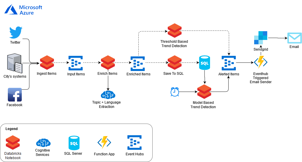
 The data flow is the following:

1. Data is arriving from either social networks or the city’s systems.
2. Events are ingested using a Spark Streaming operation (Ingest items)
3. Events are processed in external topic/language detectors. For example, Azure Text Analytics API can be employed for entity or key phrase detection. (Enrich items)
4. Incoming events are sent in parallel to two tasks: Batch and Stream
   • Batch
     1. Metadata from all enriched items is stored in a SQL server. The database stores the time, topic and additional metadata about each item, for further aggregation at a later phase. (Save to SQL)
     2. A batch operation runs every fixed period equal to the time interval selected during modeling and reads two datasets: The history (e.g. 1 month back), and events from the latest time interval.
     3. The model trains on the history time-series and predicts anomalies for the last time interval. (Model based trend detection)
   • Stream: In parallel to the batch operation, a Spark Streaming operation groups items at relatively short time intervals to detect extreme anomalies. It compares the number of items per time range to a constant. (Threshold based trend detection)
5. Predicted events are further processed in UIs or alerts such as email senders. (Alerted items)

Time series forecasting used in real time for a stream of data is inherently different from other machine learning tasks. Most models are lazy, i.e. the model is trained with the entire data to forecast the next value, and data is usually non-stationary. In a classical machine learning setting, a model is trained once and serves new samples multiple times. In the time-series scenario, the model must be trained or updated before each prediction or a small set of prediction, and predictions usually require the last k values of the time-series as features. Therefore, we use a SQL server to hold historical data and supply it to the model during inference. Some models, such as recurrent neural networks, can still be used without being trained before each sample, and some models allow an online learning setting which adapts the model for each new sample.

Discussion

By detecting trending topics, we allow municipalities, which are ZenCity’s customers, to gain insights about events in specific points in time. Municipalities which become more data driven than ever have an additional set of tools to detect, examine and act upon events occurring in their jurisdiction. They can respond to events which were previously impossible to identify and estimate the level of engagement for different activities, thus becoming better decision makers and better servants for their citizens. Moreover, fusing such data with other temporal data like sensors can provide additional insights and help the municipality better define root causes for many of the city’s problems.

Trending topics analysis is an interesting and challenging task. In its essence, it’s a hybrid text analytics and time series analysis problem. Manual labeling is difficult and subjective, and multiple labelers should be used for a robust labeled dataset. In this engagement we adapted and evaluated multiple trending topics detectors and built a pipeline to support such models at scale. We built an open source labeling tool, taganomaly, for time series anomaly detection, and developed an open source python package, moda, for running and evaluating models. We find that the best model is often dependent on the dataset characteristics, such as the time interval size, seasonality, volume of data and the accuracy of topic extractors that feed it with data.

References:

[1] Trend Detection in Social Data, a Twitter white paper [https://developer.twitter.com/content/dam/developer-twitter/pdfs-and-files/Trend%20Detection.pdf]

[2] Seasonal decomposition, In: Forecasting: Principles and practice, Rob J Hyndman and George Athanasopoulos [https://otexts.org/fpp2/components.html]

[3] Trend and Event Detection in Social Streams, Kostas Tsioutsiouliklis [http://citeseerx.ist.psu.edu/viewdoc/download?doi=10.1.1.258.9541&rep=rep1&type=pdf]

[4] STL Algorithm explained – Part II [http://www.gardner.fyi/blog/STL-Part-II/]

[5] Cleveland, William S. (1979). “Robust Locally Weighted Regression and Smoothing Scatterplots”. Journal of the American Statistical Association. 74 (368): 829–836.

Code/Data:

[6] TagAnomaly: Time series anomaly detection labeling tool [https://github.com/Microsoft/TagAnomaly]

[7] moda: Python package for detecting trending topics using time series models [https://github.com/omri374/moda]

[8] Social posts pipeline: A Databricks based pipeline for detecting trending topics at scale [https://github.com/morsh/social-posts-pipeline]

[9] San Francisco Open311 website [https://data.sfgov.org/City-Infrastructure/311-Cases/vw6y-z8j6/data]

[10] Azure Machine Learning Anomaly Detection API

[11] CI/CD story for this use case [https://www.microsoft.com/developerblog/2018/12/12/databricks-ci-cd-pipeline-using-travis]

[12] Twitter Anomaly Detection R package [https://github.com/Twitter/AnomalyDetection]

[13] 3rd Party Twitter Anomaly Detection python package [https://github.com/Marcnuth/AnomalyDetection]

 

Special thanks to the Microsoft team who worked on this project: Mor Shemesh, Tamir Kamara and Sachin Kundu, and to ZenCity’s team: Ido Ivri, Alon Nisser, Yoav Luft, Shay Palachy and Ori Cohen.