Semantic Segmentation of Small Data using Keras on an Azure Deep Learning Virtual Machine

Margaret Meehan

July 18th, 20180 0

Introduction

As previously featured on the Developer Blog, golf performance tracking startup Arccos joined forces with Commercial Software Engineering (CSE) developers in March in hopes of unveiling new improvements to their “virtual caddie” this summer. Powered by Microsoft Azure, Arccos’ virtual caddie app uses artificial intelligence to give golfers the performance edge of a real caddie. By crunching data collected from a player’s personal swing history, the virtual caddie can recommend an optimal strategy for any golf course hole anywhere in the world.

For each golf course, the virtual caddie can evaluate the impact of wind speed, elevation, and other weather patterns on a golfer’s shot. However, to optimize the caddie’s advice, the mobile app needed to better detect obstacles like trees or buildings. This is where the CSE engineers jumped in to help the Arccos engineers.

One of our previous posts explained how Microsoft developers worked with Arccos to develop a novel method for rapidly pre-labeling training data for image segmentation models. In this code story, we’ll recount our collaboration with Arccos to create a semantic segmentation model that, given a satellite image of a golf course, classifies each pixel as playable or non-playable based on the existence of obstructions such as trees. We built on previous work from an extended engagement between CSE and Arccos, which identified image segmentation as the top approach. To train our model, we started with a small dataset of less than 100 annotated satellite images. The annotations are grayscale masks where black or white indicates playable or non-playable areas, respectively.

Satellite Image and Mask

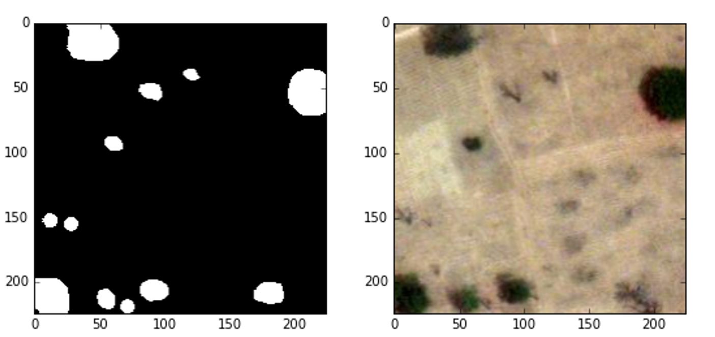
The non-playable areas denoted by white pixels correspond to trees while the remaining black pixels show playable areas without obstructions. As we cannot disclose Arccos’ data publicly, the image and its mask come from the Kaggle Dstl Satellite Imagery Feature Detection competition.

Since we aimed for state-of-the-art results, we turned to Convolutional Neural Networks (CNNs) because they have performed very well on a variety of computer vision challenges. While it would be logical to train a CNN on our dataset, many of the most performant CNNs were designed for large datasets such as COCO. When evaluating our potential solutions, we feared that training one of these models from scratch would result in overfitting to our small dataset. Therefore, if we wanted to use CNNs with known performance characteristics, we faced two choices: finding and training a model that performed well on small data or applying transfer learning techniques by leveraging a pre-trained model.

Why U-Net for Small Data?

In search of a model suited to our data, we came across the U-Net, a CNN that was created for semantic segmentation of small datasets of biomedical images from electron microscopes. While our data bears little resemblance to biomedical images, the network’s architecture does not include any design decisions that prohibit the U-Net from performing well on other types of small datasets. Rather, as top entries in the Kaggle Dstl Satellite Imagery Feature Detection competition show, the U-Net works well on satellite imagery like our aerial golf course images.

The U-Net’s architecture was inspired by Fully Convolutional Networks for Semantic Segmentation. In this paper, the authors describe how to adapt image classification models that have a convolutional base and fully connected classification layers into Fully Convolutional Networks (FCNs) capable of performing semantic segmentation. FCNs for semantic segmentation replace the fully connected layers with convolutional layers and extend the network by adding learnable upsampling layers. Unlike fully connected layers, the convolutional layers allow the network to work with arbitrarily sized images. The upsampling layers ensure that the width and height of the output mask are the same as the input image while also learning spatial information crucial to localization that would otherwise be lost if simply flattened as input into fully connected layers.

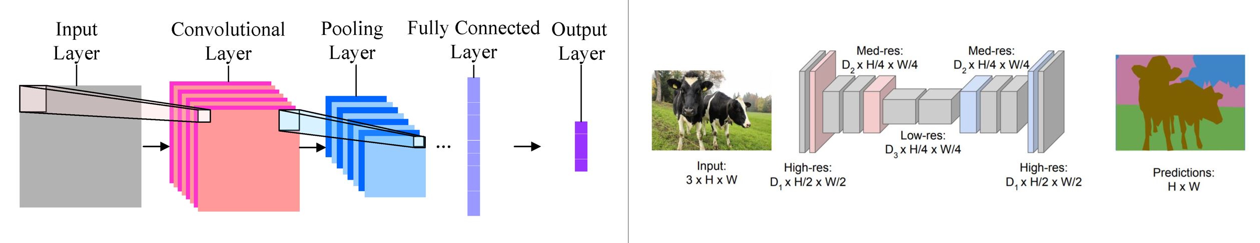
The image on the left shows a typical image classification network where the latent space is flattened into a fully connected layer before output. In contrast, the image on the right shows a FCN for semantic segmentation where the latent space is upsampled without losing spatial information by flattening.

More generally, FCNs for semantic segmentation (and therefore, the U-Net) are similar to autoencoders in that they encode a hierarchical representation of an image in a compressed latent space and decode that representation into an output with the same width and height as the input. While encoding and decoding images seems to complicate semantic segmentation since input and output dimensions share the same width and height, this process is necessary because the convolutional layers derive their representational power from their filter depth and the receptive field of those filters. The pooling layers compress the width and height so each successive layer’s filters have a larger receptive field and thus learn a representation of the entire image.

The pictured autoencoder, viewed from left to right, is a neural network that “encodes” the image into a latent space representation and “decodes” that information to reconstruct the original image.

The U-Net derives its name from the near symmetry of the encoding and decoding layers of the network that form a visual “U”, and it is this symmetry that allows the U-Net to perform so well on small data. By concatenating the output from encoder layers to their upsampled symmetric counterparts in the decoder, the U-Net can pass spatial information that is lost in the encoding process back to the decoder. Furthermore, by performing convolutions on those concatenated layers, the decoder can learn a more spatially precise output that can then be propagated to higher resolution layers.

The U-Net performs convolutions in the decoder on spatial information from both the latent space representation and the encoder.

Based on the theoretical underpinnings of the U-Net’s architecture and its success in the DSTL Kaggle competition, we decided to apply it to our data. We also considered using transfer learning with other pre-trained models. However, our intuition told us that transfer learning wouldn’t work well here because satellite images greatly differ from the standard image datasets that models are pre-trained on. Since annotating images for semantic segmentation is particularly slow and laborious, we planned to attempt transfer learning after we created a larger annotated dataset by leveraging Otsu’s method to build a tool that makes it trivial to annotate images.

Keras Implementation

When implementing the U-Net, we needed to keep in mind that it would be maintained by engineers that do not specialize in the mathematical minutia found in deep learning models. Therefore, we turned to Keras, a high-level neural networks API, written in Python and capable of running on top of a variety of backends such as TensorFlow and CNTK. Keras comes with predefined layers, sane hyperparameters, and a simple API that resembles that of the popular Python library for machine learning, scikit-learn. By choosing Keras and utilizing models built by the open source community, we created a maintainable solution that required minimal ramp-up time and allowed us to focus on the architecture of the network rather than the implementations of specific neurons.

The full model architecture demonstrates the simplicity of implementing complex neural networks in Keras. From the application programmer’s perspective, layers can be added without worrying about the implementation of the neurons that form the layer. This encourages application programmers to think about higher level concepts like tensor shapes and types of layers rather than implementation details. Keras even provides a summary function on models that will show the network’s topology from a high level perspective.

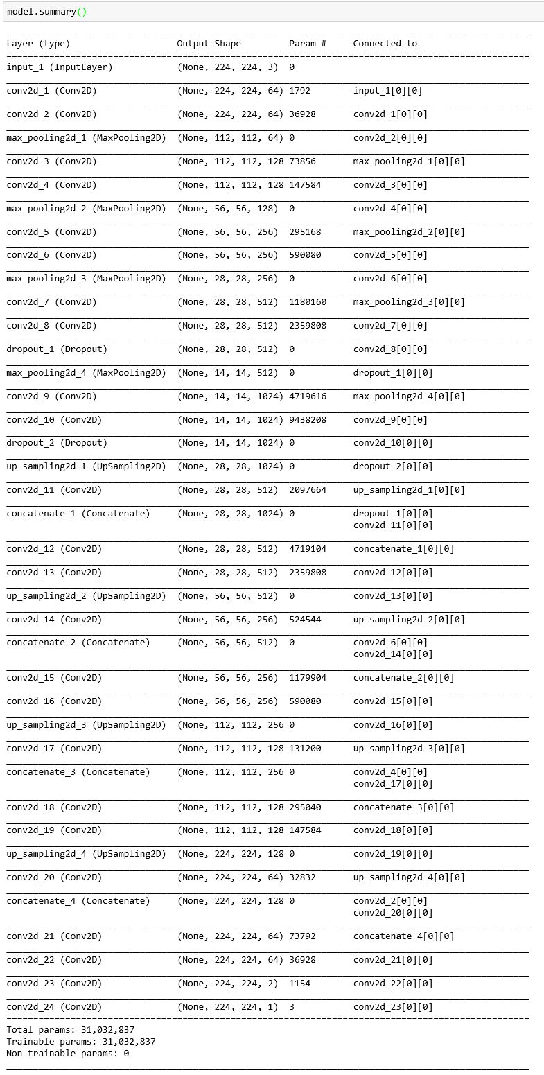
The diagram generated by model.summary() shows important high level information about the model such as the output shapes of each layer, the number of parameters, and the connections. To experiment more with this architecture, checkout our Azure Notebook.

While Keras simplifies our implementation, setting up the proper environment with Keras and its dependencies can be prohibitively challenging. Instead of manually installing all the necessary libraries for Keras, we provisioned a Deep Learning Virtual Machine (DLVM) on Azure. These GPU-based machines come with many popular tools for deep learning, including Keras and all its dependencies. By taking advantage of the DLVM, we were able to jump into development right away rather than spending our time setting up a development environment.

Training

Although Keras handles most details related to training for us, we needed to specify a loss function to minimize. In our case, each type of course, had large variations in the distributions of playable to non-playable pixels. For instance, arid courses have a lower ratio of non-playable to playable pixels because they do not have much vegetation. Similarly, lush courses have a more equal ratio of non-playable to playable pixels because they have much more vegetation. Unlike a class imbalance problem, we could not specify one penalty that would account for each type of course. Instead, we used small mini-batches and minimized the inverse of the dice coefficient. This approach accounted for the varying distribution of playable to non-playable pixels among individual images instead of penalizing misclassifications based on characteristics of the entire dataset.

The dice coefficient deals with class imbalance by accounting for both precision and recall. By choosing small mini-batches, the dice coefficient could account for the different distributions among individual images for each mini-batch instead of penalizing misclassifications based on characteristics of the entire dataset.

def dice_coef(y_true, y_pred):
    '''
    Params: y_true -- the labeled mask corresponding to an rgb image
            y_pred -- the predicted mask of an rgb image
    Returns: dice_coeff -- A metric that accounts for precision and recall
                           on the scale from 0 - 1. The closer to 1, the
                           better.
    Citation (MIT License): https://github.com/jocicmarko/
                            ultrasound-nerve-segmentation/blob/
                            master/train.py
    '''
    y_true_f = Keras.flatten(y_true)
    y_pred_f = Keras.flatten(y_pred)
    intersection = Keras.sum(y_true_f * y_pred_f)
    smooth = 1.0
    return (2.0*intersection+smooth)/(Keras.sum(y_true_f)+Keras.sum(y_pred_f)+smooth)

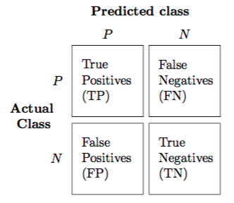
The above confusion matrix can be used to calculate precision and recall, which helps to develop an intuition behind the choice of dice coefficient. Intuitively, by minimizing the inverse of the dice coefficient, we try to achieve precision and recall values as close to 1 as possible.

On our small dataset, the trained model achieved a dice coefficient of 0.75 on the validation set. While this result proved quite successful in providing insights, there was still room for improvement. In the future, we plan on augmenting our data by generating new images from our existing dataset and tuning hyperparameters via tools like hyperopt. Additionally, once we have more labeled data, we will be able to further explore transfer learning options.

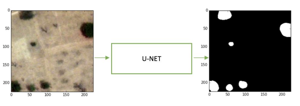
The above image shows a trained model on the Kaggle dataset. Although the model does not detect every tree as it is not perfect, it easily finds large obstructions that would inhibit golfers on the course.

Conclusion

In this post, we demonstrated a maintainable and accessible solution to semantic segmentation of small data by leveraging Azure Deep Learning Virtual Machines, Keras, and the open source community. We anticipate that the methodology will be applicable for a variety of semantic segmentation problems with small data, beyond golf course imagery.

If you would like to quickly annotate more image segmentation data, have a look at an image annotation tool based on Otsu’s method. We welcome feedback in the comments and encourage our readers to share their experiences with this methodology. As an aside, if you are experimenting with Object Detection models, our Visual Object Tagging Tool will speed up your labeling process.

Acknowledgments

Here we will give acknowledgment to several key members that contributed to solutions which were essential to this project. Thanks to Mona Habib for identifying image segmentation as the top approach and the discovery of the satellite image dataset, plus the first training of the model. Thanks to Micheleen Harris for longer-term support and engagement with Arccos, refactoring much of the image processing and training code, plus the initial operationalization. Thanks to David Crook for his leadership and technical expertise, performing much of the machine learning, and operationalization. Thanks to Beth Zeranski for her leadership and technical expertise, as well as driving our feedback into product engineering. Thanks to all for continued iterations of the solution and follow-ups with Arccos throughout this process, leading up to this very successful event.