Bird Detection with Azure ML Workbench

Olga Liakhovich

Introduction

Estimation of population trends, detection of rare species, and impact assessments are important tasks for biologists. Recently, our team had the pleasure of working with Conservation Metrics, a services provider for automated wildlife monitoring, on a project to identify red-legged kittiwakes in photos from game cameras. Our work included labeling data, model training on the Azure Machine Learning Workbench platform using Microsoft Cognitive Toolkit (CNTK) and Tensorflow, and deploying a prediction web service.

In this code story, we’ll discuss different aspects of our solution, including:

1. Data used in the project and how we labeled it
2. Object detection and Azure ML Workbench
3. Training the Birds Detection Model with CNTK and Tensorflow
4. Deployment of web services
5. Demo app setup

Data

Below is a video (provided by Abram Fleishman of San Jose State University and Conservation Metrics, Inc) capturing the native habitat of red-legged kittiwakes, species that we worked on detecting. Biologists use various pieces of equipment, including climbing gear, to install cameras on those cliffs and take daytime and nighttime photos of birds.

We used photos to train the model and The Visual Object Tagging Tool (VOTT) was helpful with labeling images. It took about  20 hours to label the data and close to 12,000 bounding boxes were marked.

The labeled data can be found in this GitHub repo.

Data Credit

This data was collected by Dr. Rachael Orben of Oregon State University and Abram Fleishman of San Jose State University and Conservation Metrics, Inc. as part of a large project investigating early breeding season responses of red-legged kittiwakes to changes in prey availability and linkages to the non-breeding stage in the Bering Sea, Alaska.

Introduction to Object Detection

For a walkthrough on object detection techniques, please refer to this blog post on CNNs. Faster R-CNNs (Region proposals with Convolutional Neural Networks) are a relatively new approach (the first paper on this approach was published in 2015). They have been widely adopted in the Machine Learning community, and now have implementations in most of popular Deep Neural Net frameworks (DNNs) including PyTorch, CNTK, Tensorflow, Caffe, and others.

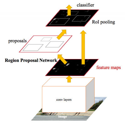
In this post, we will cover the Faster R-CNN object detection APIs provided by CNTK and Tensorflow.

Azure Machine Learning Workbench

For model training and the creation of prediction web services, we explored the recently-announced Azure Machine Learning Workbench, which is an analytics toolset enabling data scientists to prepare data, run machine learning training experiments and deploy models at cloud scale (see setup and installation documentation).

As we’ll be working with an image-related scenario, we’ve used the CNTK and Tensorflow MNIST  handwritten digit classification templates that ship with the tool as a starting point for our experimentation.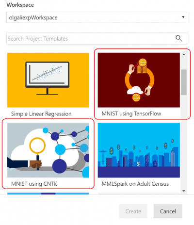 

DNN training usually benefits from running on GPUs that allow the required matrix operation to run much faster. We provisioned Data Science VMs with GPUs and used the remote Docker execution environment that Azure ML Workbench provides (see details and more information on execution targets) for training models.

Azure ML logs the results of jobs (experiments) in a run history. This capability was quite useful as we experimented with various model parameter settings, as it gives a visual means to select the model with the best performance. Note that you need to add instrumentation using Azure ML Logging API to your training/evaluation code and track metrics of interest (for example, classification accuracy).

Image Labeling and Exporting

We used the VOTT utility (available for Windows and MacOS) to label and export data to CNTK and Tensorflow Pascal formats, respectively.

The tool provides a friendly interface for identifying and tagging regions of interest in images and videos. Using it requires collecting the images in a folder, then simple Launch VOTT, point to the image dataset, and proceed to label the regions of interest.

When finished, click on Object Detection, then Export Tags to export to CNTK and Tensorflow.

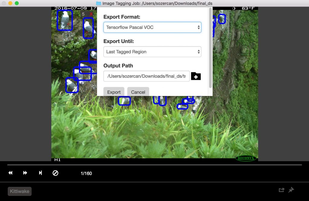
For Tensorflow, VOC Pascal is the export format, so we converted the data to TFRecords to be able to use it in training and evaluation. For details, see the section on Tensorflow below.

Training Birds Detection Model with CNTK

As mentioned in the previous section, we used the popular Faster R-CNN approach in our Birds Detection model. You may wish to read CNTK’s documentation about object detection using Faster R-CNN for more information. In this section, we are going to focus on two parts of our approach.

1. Using Azure ML Workbench to start training on remote VM
2. Hyperparameter tuning through Azure ML Workbench

Using Azure ML Workbench for Training on a Remote VM

Hyperparameter tuning is a major part of the effort to build a production-ready machine learning (or deep learning) models after the first draft model is created that shows promising results. Our problem here is to accomplish it efficiently and using Azure ML Workbench to facilitate the process.

Parameter tuning requires a large number of training experiments, typically a time-consuming process. One approach is to train on a powerful local machine or cluster. Our approach, however, is to take training into the cloud by using Docker containers on remote (virtual) machines. The key advantage is that we can now spin off as many containers we want to tune parameters in parallel. Based on this documentation for Azure ML,  register each VM as a compute target for the experiment. Note that there are constraints on password characters; for example, using “*” in the password will produce an error.

az ml computetarget attach --name "my_dsvm" --address "my_dsvm_ip_address" --username "my_name" --password "my_password" --type remotedocker

After the command is executed, myvm.compute and myvm.rucomfig are created in the aml_config folder. Since our task is better suited to a GPU machine, we have to make some following modifications:

In myvm.compute

baseDockerImage: microsoft/mmlspark:plus-gpu-0.7.91
nvidiaDocker: true

In myvm.runconfig

EnvironmentVariables:
    "STORAGE_ACCOUNT_NAME": 
    "STORAGE_ACCOUNT_KEY": 
Framework: Python
PrepareEnvironment: true

We used Azure storage for storing training data, pre-trained models and model checkpoints. The storage account credentials are provided as EnvironmentVariables. Be sure to include the necessary packages in conda_dependencies.yml

Now we can execute the command to start preparing the machine.

az ml experiment –c prepare myvm

Followed by training our object detection model.

az ml experiment submit –c Detection/FasterRCNN/run_faster_rcnn.py
..
..
..
Evaluating Faster R-CNN model for 53 images.
Number of rois before non-maximum suppression: 8099
Number of rois  after non-maximum suppression: 1871
AP for       Kittiwake = 0.7544
Mean AP = 0.7544

Hyperparameter Tuning with Azure ML Workbench

With the help of Azure ML and Workbench, it’s easy to log the hyperparameters and different performance metrics while spinning up several containers to run in parallel (read more about logging detail information in the documentation).

The first approach to try is different pre-trained base models. At the time of writing this post, CNTK’s Faster R-CNN API supported two base models: AlexNet and VGG16. We can use these trained models to extract image features. Though these base models are trained on different datasets like ImageNet, low- and mid-level image features are common across applications and are therefore shareable. This phenomenon is called “transfer learning.” AlexNet has 5 CONV (convolution) layers while VGG16 has 12 CONV layers. In terms of the number of trainable parameters, VGG16 has 138 million, roughly three times more than AlexNet; we used VGG16 as our base model here. The following are the VGG16 hyperparameters we optimized to achieve the best performance out of our evaluation set.

In Detection/FasterRCNN/FasterRCNN_config.py:

# Learning parameters
__C.CNTK.L2_REG_WEIGHT = 0.0005
__C.CNTK.MOMENTUM_PER_MB = 0.9
# The learning rate multiplier for all bias weights
__C.CNTK.BIAS_LR_MULT = 2.0

In Detection/utils/configs/VGG16_config.py:

__C.MODEL.E2E_LR_FACTOR = 1.0
__C.MODEL.RPN_LR_FACTOR = 1.0
__C.MODEL.FRCN_LR_FACTOR = 1.0

Azure ML Workbench definitely makes visualizing and comparing different parameter configurations easier.

mAP using VGG16 base model

Evaluating Faster R-CNN model for 53 images.
Number of rois before non-maximum suppression: 6998
Number of rois  after non-maximum suppression: 2240
AP for       Kittiwake = 0.8204
Mean AP = 0.8204

Please see the GitHub repo for the implementation.

Training Birds Detection Model with Tensorflow

Google recently released a powerful set of object detection APIs. We used their documentation on how to train a pet detector with Google’s Cloud Machine Learning Engine as inspiration for our project to train our kittiwake bird detection model on Azure ML Workbench. The Tensorflow Object Detection API has a variety of pre-trained models on the COCO dataset. In our experiments, we used ResNet-101 (Deep Residual Network with 101 layers) as a base model and used the pets detection sample config as a starting point for object detection training configuration.

This repository contains the scripts we used for training objected detection models with Azure ML Workbench and Tensorflow.

Setting Up Training

Step 1: Prepare data in the TF Records format required by Tensorflow’s object detection API. This approch requires that we convert the default output provided by the VOTT tool. See details in the generic converter, create_pascal_tf_record.py.

python create_pascal_tf_record.py 
    --label_map_path=/data/pascal_label_map.pbtxt 
    --data_dir=/data/ 
    --output_path=/data/out/pascal_train.record 
    --set=train

python create_pascal_tf_record.py 
    --label_map_path=/data/pascal_label_map.pbtxt 
    --data_dir=/data/ 
    --output_path=/data/out/pascal_val.record 
    --set=val

Step 2: Package the Tensorflow Object Detection and Slim code so they can be installed later in the Docker image used for experimentation.  Here are the steps from Tensorflow’s Object Detection documentation:

# From tensorflow/models/research/
 python setup.py sdist
 (cd slim && python setup.py sdist)

Next, move the produced tar files to a location available to your experimentation job (for example, blob storage) and put a link in the conda_dependancies.yaml for your experiment.

dependencies:
-python=3.5.2
-tensorflow-gpu
-pip:
  #... More dependencies here…
  #TF Object Detection
  -https:///object_detection-0.1.tar.gz
  -https:////slim-0.1.tar.gz

Step 3: In your experiment drive script, add import

from object_detection.train import main as training_module

Then you can invoke training routing in your code with training_module(_).

Training and Evaluation Flow

The Tensorflow Object Detection API assumes that you will run training and evaluation (verification of how well is model performing so far) as separate calls from the command line. When running multiple experiments it may be beneficial to run evaluation periodically (for example, every 100 iterations) to get insights as to how well the model can detect objects in unseen data.

In this fork of Tensorflow Object Detection AP, we’ve added train_eval.py, which demonstrates this continuous train and evaluation approach.

 print("Total number of training steps {}".format(train_config.num_steps))
 print("Evaluation will run every {} steps".format(FLAGS.eval_every_n_steps))
 train_config.num_steps = current_step
 while current_step <= total_num_steps:
   print("Training steps # {0}".format(current_step))
   trainer.train(create_input_dict_fn, model_fn, train_config, master, task,
   FLAGS.num_clones, worker_replicas, FLAGS.clone_on_cpu, ps_tasks,
   worker_job_name, is_chief, FLAGS.train_dir)
   tf.reset_default_graph()
   evaluate_step()
   tf.reset_default_graph()
   current_step = current_step + FLAGS.eval_every_n_steps
   train_config.num_steps = current_step

To explore several hyperparameters of the model and estimate its effect on the model we split the data into train, validation (or development) and test sets of 160 images, 54 and 55 images, respectively.

Comparing Runs

The Tensorflow object detection framework provides the user with many parameter options to explore to see what works best on a given dataset.

In this exercise, we will do a couple of runs and see which one will give us the best model performance.  We will use object detection precision, usually referenced as mAP (Mean Average Precision) as our target metric. For each run, we will use azureml.logging to report the maximum value of mAP and which training iteration it was observed on. In addition, we will plot chart “mAP vs Iterations”, then save it to the output folder to be displayed in Azure ML Workbench.

Integration of  TensorBoard events with Azure ML Workbench

TensorBoard is a powerful tool for debugging and visualizing DNNs. The Tensorflow Object Detection API already emits summary metrics for Precision. In this project, we integrated Tensorflow summary events, which TensorBoard uses for its visualizations, with Azure ML Workbench.

from tensorboard.backend.event_processing import event_accumulator
from azureml.logging import get_azureml_logger

ea = event_accumulator.EventAccumulator(eval_path, ...)
df = pd.DataFrame(ea.Scalars('Precision/mAP@0.5IOU'))
max_vals = df.loc[df["value"].idxmax()]

#Plot chart of how mAP changers as training progresses
fig = plt.figure(figsize=(6, 5), dpi=75)
 plt.plot(df["step"], df["value"])
 plt.plot(max_vals["step"], max_vals["value"], "g+", mew=2, ms=10)
 fig.savefig("./outputs/mAP.png", bbox_inches='tight')

# Log to AML Workbench best mAP of the run with corresponding iteration N
 run_logger = get_azureml_logger()
 run_logger.log("max_mAP", max_vals["value"])
 run_logger.log("max_mAP_interation#", max_vals["step"])

For more details, see the code in results_logger.py.

Here is an analysis of several training runs we’ve done using Azure ML Workbench experimentation infrastructure.

Run #1 uses Stochastic Gradient Descent and data augmentation is turned off. (See this blog post for an overview of gradient optimization options.)

From the run history in Azure ML Workbench, we can see details on every run:

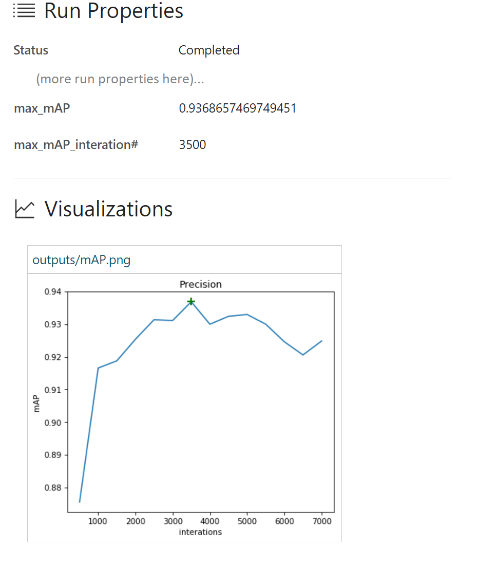
Here we see that we have achieved a maximum mAP of 93.37% around iteration #3500. Thereafter the model started overfitting to the training data and performance on the test set started to drop.

Run #2 uses the more advanced Adam Optimizer. All other parameters are the same.

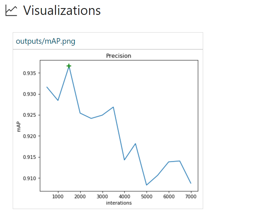
Here we reached a mAP of 93.6% much faster than in Run #1. It also seems that the model starts to overfit much sooner as Precision on the evaluation set drops quite rapidly.

Run #3 adds data augmentation to training configuration. We will stick with Adam Optimizer for all subsequent runs.

data_augmentation_options{
  random_horizontal_flip{}
}

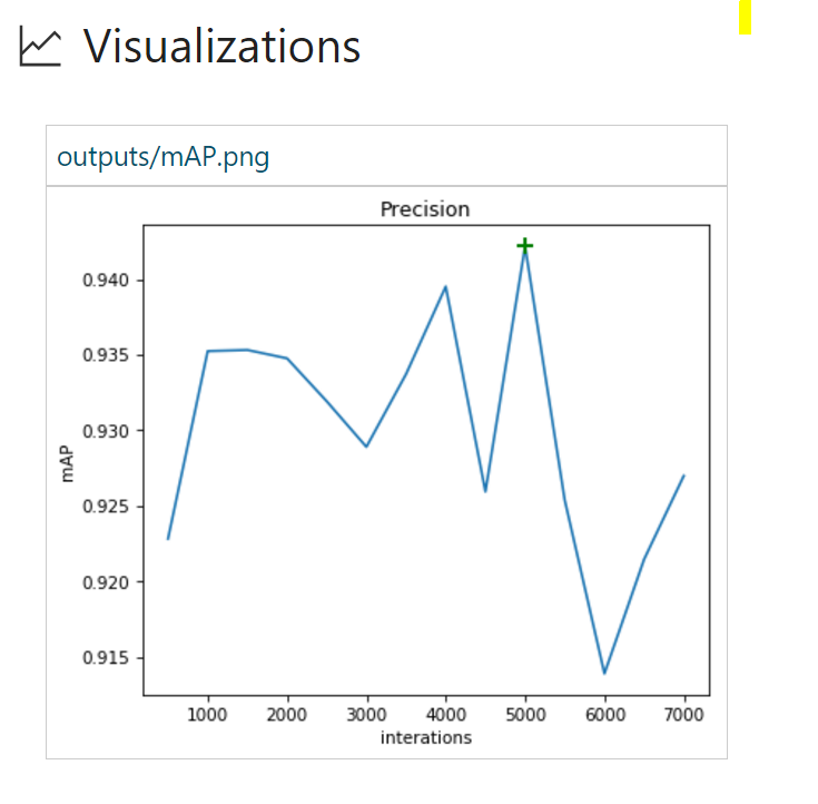
Random horizontal flipping of the images helped to improve mAP from 93.6 on Run #2  to 94.2%. It also takes more iterations for the model to start overfitting.

Run #4 involves the addition of even more data augmentation options.

data_augmentation_options{
  random_horizontal_flip{}
  random_pixel_value_scale{}
  random_crop_image{}
}

Interesting results are shown below:

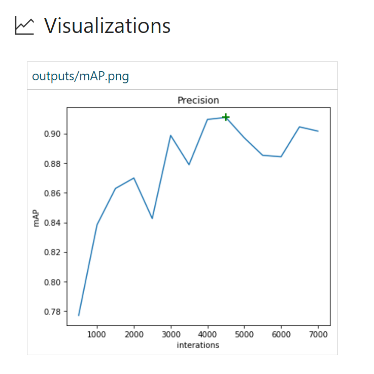
Though the mAP we are seeing here is not the greatest (91.1%), it also did not overfit after 7,000 iterations. A natural follow-up could be to train this model even longer and see if there is still the potential to get to a higher mAP.

Here is an at-a-glance view of our training progress from Azure ML Workbench:

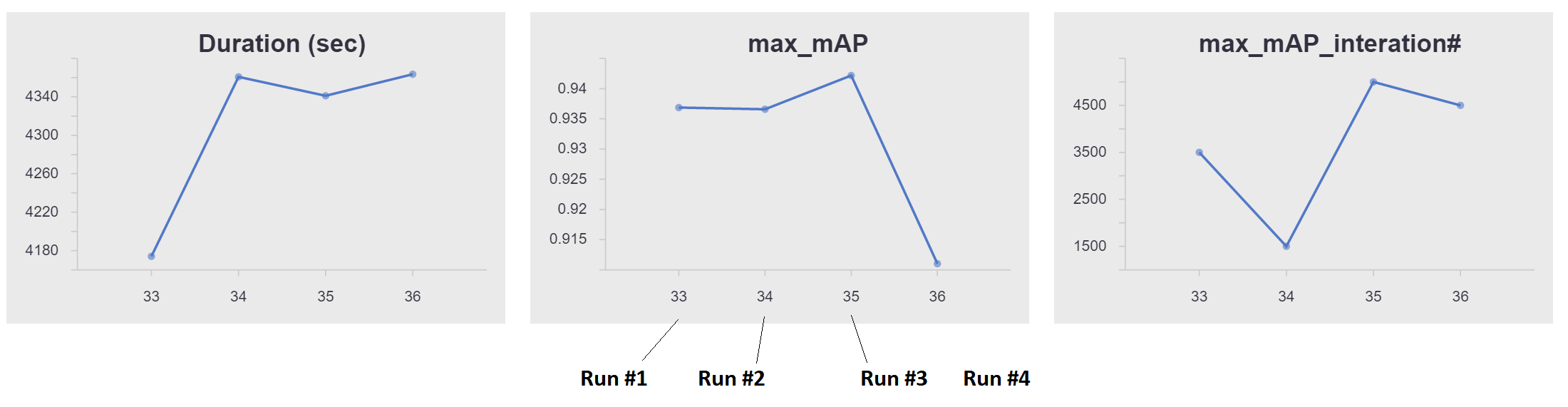
Azure ML Workbench allows users to compare runs side by side (below are Run 1, 3 and 4):

We can also plot evaluation results on image(s) of interest and use those, too, when comparing results. TensorBoard events already have all the required data.

In summary, ResNet-powered object detection allowed us to achieve great results even on smaller datasets. Azure ML Workbench provided a useful infrastructure so we could have a central place for all experiment execution and results comparisons.

Deploying Scoring Web Service

After developing an object detection and classification model with satisfactory performance, we proceeded to deploy the model as a hosted web service so that it can be consumed by the bird-monitoring application in the solution pipeline. We’ll show how that can be done using the built-in capabilities provided by Azure ML, and also as a custom deployment.

Web Service Using Azure ML CLI

Azure ML provides extensive support for model operationalization on local machines or the Azure cloud.

Installing Azure ML CLI

To get started on deploying your model as a web service, first, we will need to SSH into the VM we are using.

ssh @

In this example, we will be using an Azure Data Science VM that already has Azure CLI installed. If you are using another VM, you can install Azure CLI using:

pip install azure-cli
pip install azure-cli-ml

Log in using:

az login

Setting Up the Environment

Let’s start by registering the environment provider by using:

az provider register -n Microsoft.MachineLearningCompute

For deploying the web service on a local machine, we’ll have to set up the environment first:

az ml env setup -l [Azure region, e.g. eastus2] -n [environment name] -g [resource group]

This step will create the resource group, storage account, Azure Container Registry (ACR), and Application Insights account.

Set the environment to the one we just created:

az ml env set -n [environment name] -g [resource group]

Create a Model Management account:

az ml account modelmanagement create -l [Azure region, e.g. eastus2] -n [your account name] -g [resource group name] --sku-instances [number of instances, e.g. 1] --sku-name [Pricing tier for example S1]

We are now ready to deploy the model! We can create the service using:

az ml service create realtime --model-file [model file/folder path] -f [scoring file e.g. score.py] -n [your service name] -r [runtime for the Docker container e.g. spark-py or python] -c [conda dependencies file for additional python packages]

Please note that nvidia-docker is not supported for prediction right now. Make sure to edit your Conda dependencies to remove any GPU-specific references like tensorflow-gpu.

After deploying the service, you can access information on how to use the web service with:

az ml service usage realtime -i [your service name]

For example, you can test the service using curl with:

curl -X POST -H "Content-Type:application/json" --data !! YOUR DATA HERE !! http://127.0.0.1:32769/score

Alternative Option to Deploy Scoring Web Service

Another way to deploy a web service to serve predictions is to create your own instance of Sanic web server. Sanic is a Flask-like Python 3.5+ web server that helps us create and run web applications. We can use the model we have trained in the previous section using CNTK and Faster R-CNN to serve predictions to identify the location of a bird within an image.

First, we need to create a Sanic web application. You can follow the code snippets below (and app.py) to create a web application and define where it should run on the server. For each API you want to support, you can also define routes, HTTP methods, and ways to handle each request.

app = Sanic(__name__)
 Config.KEEP_ALIVE = False

server = Server()
 server.set_model()

@app.route('/')
 async def test(request):
 return text(server.server_running())

@app.route('/predict', methods=["POST",])
 def post_json(request):
 return json(server.predict(request))

app.run(host= '0.0.0.0', port=80)
 print ('exiting...')
 sys.exit(0)

Once we have the web application defined, we need to build our logic to take the path of an image and return the predicted results to the user.

From predict.py, we first download the image that needs to be predicted, then evaluate that image against the previously trained model to return JSON of predicted results.

regressed_rois, cls_probs = evaluate_single_image(eval_model, img_path, cfg)
bboxes, labels, scores = filter_results(regressed_rois, cls_probs, cfg)

The returned JSON is an array of predicted labels and bounding boxes for each bird that is detected in the image:

[{"label": "Kittiwake", "score": "0.963", "box": [246, 414, 285, 466]},...]

Now that we have implemented the prediction logic and the web service, we can host this application on a server. We will use Docker to make sure our deployment dependencies and process are both easy and repeatable.

cd CNTK_faster-rcnn/Detection

Create a Docker image with a Dockerfile so we can run the application as a Docker container:

FROM hsienting/dl_az

COPY ./ /app
ADD run.sh /app/
RUN chmod +x /app/run.sh

ENV STORAGE_ACCOUNT_NAME 
ENV STORAGE_ACCOUNT_KEY 
ENV AZUREML_NATIVE_SHARE_DIRECTORY /cmcntk
ENV TESTIMAGESCONTAINER data

EXPOSE 80

ENTRYPOINT ["/app/run.sh"]

Now we are ready to build the Docker image by running:

docker build -t cmcntk .

Once we have the Docker image cmcntk locally, we can now run instances of it as containers. With the command below we are mounting the host volume to cmcntk in the container to persist the data (this is where we kept the model trained in the previous step). Then we map host port 80 to container port 80, and run the latest docker image cncntk.

docker run -v /:/cmcntk -p 80:80 -it cmcntk:latest

Now we can test the web service using a curl command:

curl -X POST http://localhost/predict -H 'content-type: application/json' 
-d '{"filename": ""}'

Exposing Your Services

At this point our services are running, but now what? How does a client interact them? How do we unify them under a single API? During our work with Conservation Metrics, we created an application as proof of concept to execute the entire classification pipeline.

Problem

We know what we want to do with our application, but there are a few limitations with our current services which will restrict how we can communicate with them. These include:

• Multiple services which share the same purpose (outputting label data) but do not share the same endpoint
• Exposing these services directly to the client requires CORS permissions which would have to be managed across all servers/load-balancers

Solution

To create a unified API endpoint, we’ll set up an Azure API Management Service. With this, we can set up and expose CORS-enabled endpoints for our APIs.

Azure API Management Services

Getting Started

1. Go to https://ms.portal.azure.com/#create/hub
2. Search and select for ‘API management’
3. Create and configure your instance to your liking

Configuration

Create a new API

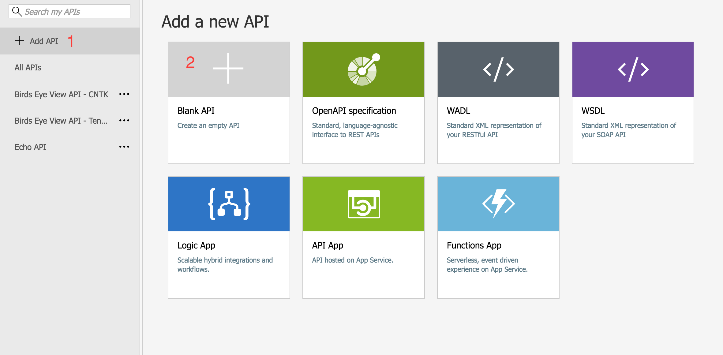
Initial configuration of your API

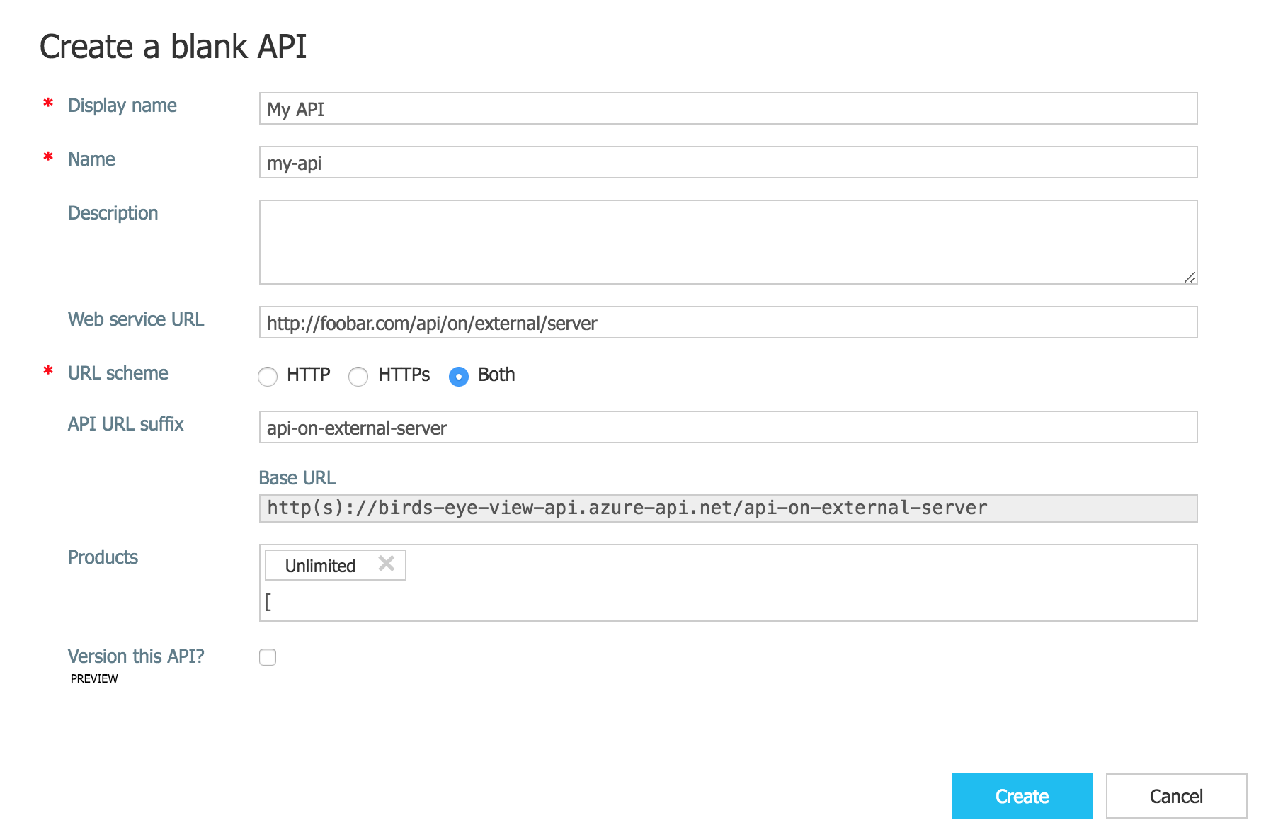
Once provisioned, go into your API. Click the “+Add API” button then the “Blank API” option. Set up the API to your liking, with Web service URL being the API on the external server, API URL suffix being the suffix which will be appended to your API Management URL, and Products being the API product type you want to register this endpoint under.

With the newly created API, configure the “Inbound processing” using the “Code View” and (to enable CORS for all external URLS) set your policies to:

    
        
        
            
                *
            
            
                *

You can now treat the API URL Suffix you set up on your API Management Service just as how you would ping our API directly.

Although there are examples from the old Azure Management Portal, you may also want to explore a more in-depth getting started guide to API Management services and CORS.

A Sample App

Our sample client web application executes the following steps:

1. Reads containers/blobs directly from Azure Blob Storage
2. Pings our new Azure API Management Service with images from our blob storage
3. Displays the returned prediction (bounding boxes for birds) on the image

You can find the code on GitHub.

Pinging the API Management Service

The only difference in pinging your API Management services, as opposed to your native API, is that you’ll have to include an additional Ocp-Apim-Subscription-Key header in all your requests. This subscription key is bound to your API Management Product, which is an accumulation of the API endpoints you release under it.

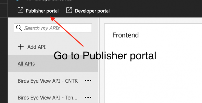
To get your Subscription Key:

1. Go to your API’s “Publisher Portal”
2. Select your desired user under the Users Menu item
3. Note the subscription key you wish to use

In this sample application, we now append this subscription key as the value for the now-attached Ocp-Apim-Subscription-Key header:

export async function cntk(filename) {
  return fetch('/tensorflow/', {
    method: 'post',
    headers: {
      Accept: 'application/json',
      'Content-Type': 'application/json',
      'Cache-Control': 'no-cache',
      'Ocp-Apim-Trace': 'true',
      'Ocp-Apim-Subscription-Key': ,
    },
    body: JSON.stringify({
      filename,
    }),
  })
}

Using The Data

You now have the ability to ping your services with an image and get a list of bounding boxes returned.

The basic use case is to just draw the boxes onto the image. One simple way to do this on a web client is to display the image and overlay the boxes using the .

<body>
  <canvas id='myCanvas'></canvas>
  <script>
    const imageUrl = "some image URL";
    cntk(imageUrl).then(labels => {
      const canvas = document.getElementById('myCanvas')
      const image = document.createElement('img');
      image.setAttribute('crossOrigin', 'Anonymous');
      image.onload = () => {
        if (canvas) {
          const canvasWidth = 850;
          const scale = canvasWidth / image.width;
          const canvasHeight = image.height * scale;
          canvas.width = canvasWidth;
          canvas.height = canvasHeight;
          const ctx = canvas.getContext('2d');

          // render image on convas and draw the square labels
          ctx.drawImage(image, 0, 0, canvasWidth, canvasHeight);
          ctx.lineWidth = 5;
          labels.forEach((label) => {
            ctx.strokeStyle = label.color || 'black';
            ctx.strokeRect(label.x, label.y, label.width, label.height);
          });
        }
      };
      image.src = imageUrl;
    });
  </script>
</body>
</html>

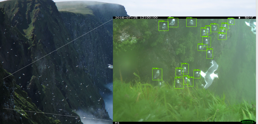
This code will propagate on your canvas with something like the image below:

Now you can interact with your trained model and demo prediction results! For code details, please refer to this GitHub repo.

Summary

In this post, we have covered our end-to-end flow for object detection, including:

• Labeling data
• Training  CNTK/Tensorflow object detection using Azure ML Workbench
• Comparing experiment runs in Azure ML Workbench
• Model operationalization and deployment of a prediction web service
• Demo application  for making predictions

Resources

• Project’s GitHub repo.
• Azure Machine Learning Workbench documentation
• Microsoft Cognitive Toolkit Object Detection GitHub repo
• Tensorflow Object Detection API GitHub repo

Cover image provided by Conservation Metrics.

Olga Liakhovich

Follow