
IoT Sports Sensor Machine Learning Helps Amateurs Up Their Game
Recently, Microsoft partnered with the Professional Ski Instructors of America and the American Association of Snowboard Instructors, (PSIA-AASI) to use wearable IoT sensors in order to develop a machine learning model of skiing skills and expertise levels. PSIA-AASI continually evaluates new technology and methods for nurturing learning experiences for developing skiers and snowboarders.
IoT Human Sensor Data Enables Skill Measurement
Watching a professional skier practicing drills, it’s easy to recognize their expertise level. Our challenge was to create data to help characterize this expertise level. With wearable IoT sensors, we can collect positional and motion data that allow us to measure this expertise level distinction between professionals and amateurs with high precision and accuracy. In our analysis, we discovered the sensor data from just nine body positions provides ample signal to generate distinct activity signatures for the professional skiers when compared with the amateurs.
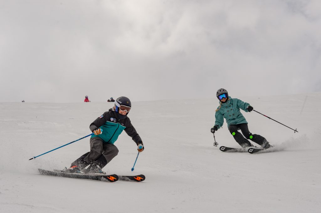
Examining the sensor data, one can see the pros’ tight adherence to proper form throughout the skill, lack of erratic movement, and precision in execution. These distinct differences in absolute and relative measures of these nine body positions allow us to construct a powerful and simple classification model to categorize skiers into different expertise levels.
We think this type of classification model can be used by the amateur to help them understand differences between their performance and that of the pro, and allow them to improve overall form and skill execution. Ski and snowboard instructors can customize training strategies for each trainee, based on the insights provided by the model and the quantitative data analysis. As a result, training can become more efficient. Over time, and with more data, more models can be created to differentiate finer-grained expertise and skill execution levels.
Data Gathering to Sports Activity Machine Learning
With PSIA-AASI, we wanted to allow amateurs to compare their own skiing data to the pros’ and classify their skill level, as well as to examine specific positional and gestural differences in their skill performance. The Microsoft and PSIA-AASI teams worked together at the Snowbird ski resort to gather the field data and build the concrete data model that would give aspiring amateurs guidance on how to improve. In this code story, we’ll describe the steps we took to gather the data and develop the model. We’ll also provide links to the R script and data set that you can use to recreate this solution.
IoT Device and Raw Sensor Data
Each of the wearable IoT sensors measures position, acceleration, and rotation individually, and records it with a time stamp. The variables emitted include positional variables x, y and z that represent position in three-dimensional space; rotational matrix variables qW, qX, qY, qZ that represent 3D rotation; and aX, aY and aZ that represent coordinate acceleration.
While the sample rate of sensors varies, we found 100 Hz to be a minimum rate for modeling. There are a number of IoT sensors that capture these data at this sample rate (more details on hardware options).
Below is an example of the raw data variables emitted by each one of the sensors.
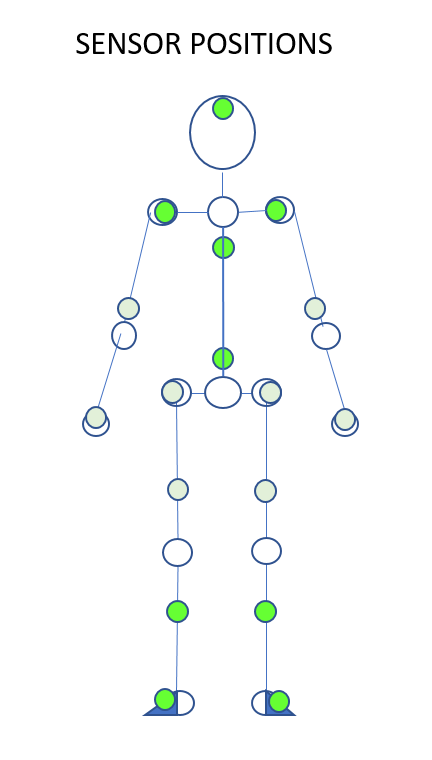
Human Sensor Placement
We placed the sensors according to the diagram included below. The data from the bright green sensors were used in the final classification model, as features generated from these sensors’ data were highly predictive of skier expertise. The features derived from the light green colored sensors’ data were not as predictive and were discarded from the final model.
We calibrated the sensors to align the timestamp for each sampling before gathering data. If you cannot calibrate sensors prior to data gathering, this manual timestamp alignment can be done as a post-processing step, presuming the sampling rate was high enough, and there is minimal missing signal. For reference, here is a time align R script example.
Experimental Design
We set out to capture data for several PSIA-AASI professional-level skiers and several intermediate skiers as they performed a number of skill drills. Our skill drills included short, medium and large radius turns. We noted the start of the actual drill in order to exclude non-drill data from the data model. We also noted the name, drill and skill level of the skier in order to annotate the data file later.
We stored our experimental data locally, then batch uploaded it to an Azure SQL database after the experiments were complete. We also tested devices using Bluetooth to stream the data to a mobile device carried by the skier, though in modeling we only used the locally stored data as we didn’t have a time constraint requiring real-time streaming, and the locally stored data had no data loss.
Clean and Transform the Data
We wrote our data to Azure SQL, and applied experiment and athlete label data, then imported it into the Azure Machine Learning workspace for the rest of the data transformation and modeling. Options for AML data import include Azure SQL Database, Azure Blob Storage, Azure Table, Azure Document DB and others.
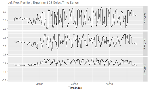
Originally, the data was saved in a “long” format, meaning that every row in the dataset represents readings from a sensor at one sampling time stamp. You can see the time series graph of each of these rows above. If we had five sensors, there would be five rows of records for each sampling time stamp. This data format presents some challenges for data analysis and modeling. We transformed this raw “long” data into the “wide” data format, with one row for each athlete and experiment. Refer to the R script for the specific code we used for this transformation, as well as the transformations and modeling that follow.
Generate Virtual Sensory Data from Physical Sensors
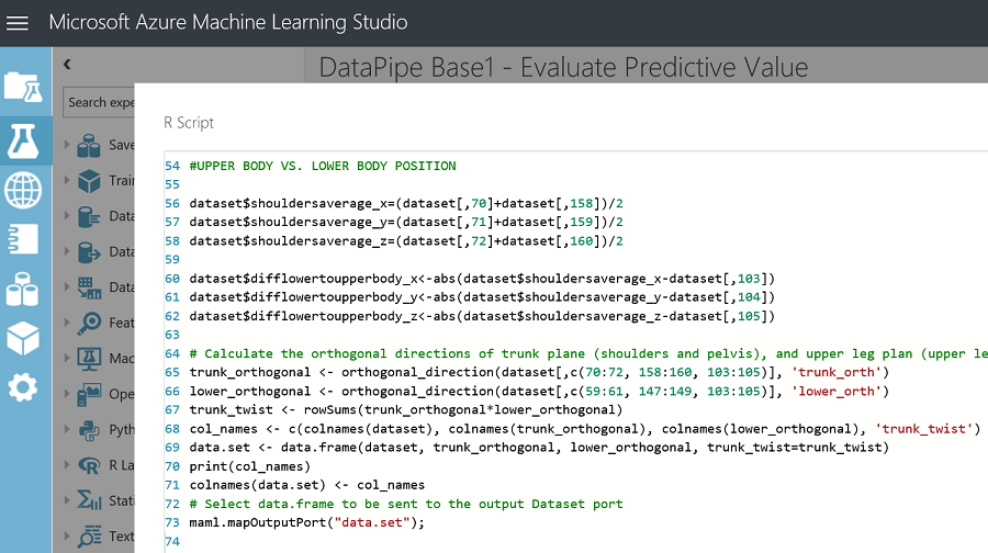
With guidance from the PSIA-AASI professionals, we characterized what hallmark differences might be captured between the pros and amateurs in the sensor data. These differences included the relative position of their upper body vs. lower body, the relative position of each of their legs and feet, and how they took a turn. With this domain expert insight, we generate virtual sensory data from the raw physical sensors that characterize limb position relative to one another, and the upper body relative to the lower body.
Later on, at the data analysis and modeling stage, we learned the features that best illustrate these differences in skiing include the normalized difference between upper body and lower body, the relational positions and rotation of upper body and lower body, and the relational position and rotation of the limbs. The screenshot below shows a few of these engineered features. You can find all the extra virtual sensory data we created in the R script.
Engineer Features by Generating Periodic Descriptive Measures
Next, we broke our ski activity sample into small activity interval slices; in our case, time slices of two seconds apiece. We generated summary statistics as well as frequency and frequency covariance statistics over these time windows. We then ran a fast-discrete Fourier transform function on each of the raw sensory signals to convert the data from being represented in a time domain to being represented in a frequency domain. This is measured by the magnitude of each frequency (from 0Hz to half of the sample frequency, 240Hz) for a given time interval slice. These generated frequency components of our sensor signal include constant power (frequency 0), low-band average power (1-40Hz), mid-band average power (41-80Hz), and high-band average power (81-120Hz). Finally, we generated cross-correlation measures on select variables to measure the similarity of various two series combinations (for more details, see the R script of this feature engineering).
Create a Classification ML Model
After feature engineering, we had 589 observations and 2144 features. Training a machine learning model with such a wide data set with so few observations would have introduced over-fitting problems, even using the simplest logistic regression model. So, we first used ‘Filter Based Feature Selection’ in Azure ML to select the top thirty features, based on strength of their relationship with the target variable, ‘SkillLevel’, as measured by Mutual Information. We did the feature selection only on the training data, which is a randomly selected 70% of the original dataset. The remaining 30% of records were held out from the feature selection and model training to be used as validation data.
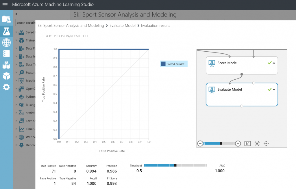
When we tested the model on the validation data, we found the model correctly predicted classification of professional vs. amateur expertise levels across all skills 99% of the time.
Access the R Script and the Full Experiment
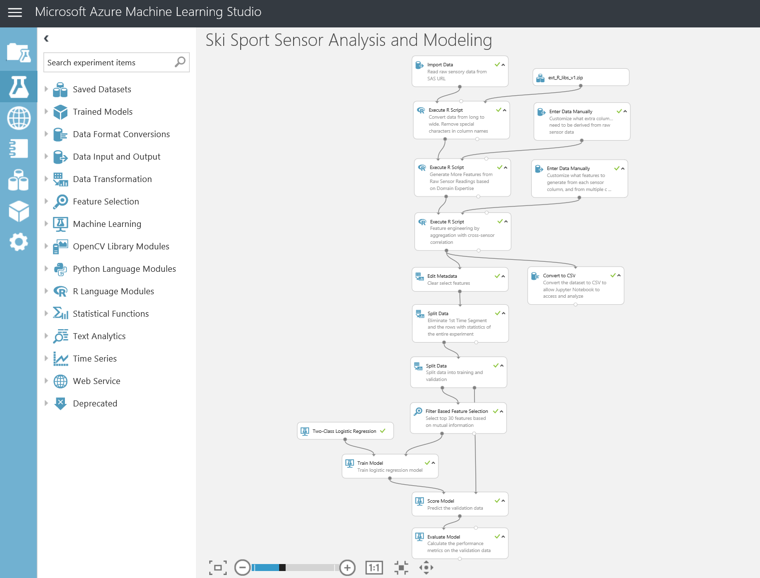
The entire R script can be accessed on GitHub. The end-to-end pipeline, including the data transformations, feature engineering, feature selection and machine learning model training and validation has been implemented in an Azure Machine Learning experiment and published in the Cortana Intelligence Suite Gallery. With this gallery experiment, you can reproduce the results presented here.
Animate Sensor Data with Avatars
For even more insight, you can turn your sensor data into your own action avatar and compare it with avatars from the pros’ sensor data.
We processed the data into a 3D skeletal animation format and imported the data into the Unity development environment to create the video you see below. We relied on the Humanoid Animation Retarget system to create a visual representation of a skier drill. In addition to this video, the 3D animation can be visualized from different perspectives and angles to better understand differences of the amateur on the left and one of the professionals on the right in terms of body positioning.
Try It Out Yourself with our IoT Sensor Data
We invite sports enthusiasts and those interested in IoT Machine Learning to analyze the full raw data set (~1.4 GB) and build the classification model for themselves. Since data transformations and feature engineering on the full raw sensor data set take some time (more than a couple of hours), we also share the smaller feature engineered dataset (~22MB) for your convenience.
Drill into Specific Comparisons
In addition to the expertise classification information, the amateur can receive guidance on areas for improvement by investigating their own skiing differences with the professionals’ performance against specific measures.
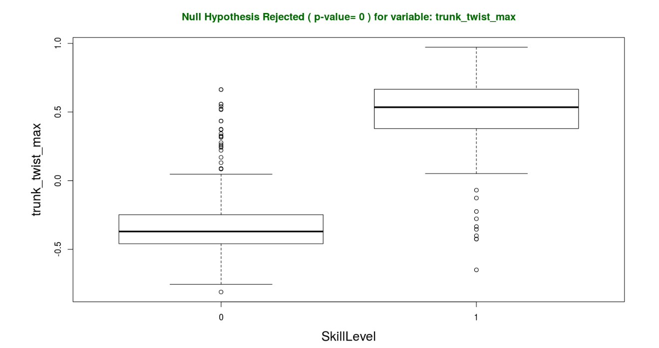
Here is an example of insights you can get from the data analysis. The variable depicted here, ‘trunk_twist_max’ is a feature we developed to measure the angle between the upper trunk (a plane spanned by both shoulders and pelvis), and the lower trunk (a plane spanned by both lower legs and pelvis). In this case, a positive value means the angle is smaller than ninety degrees. From this visualization, you can instantly tell that the professional skiers (SkillLevel of 1) hold more of a crouching pose, and the amateur skiers (SkillLevel of 0) have more of a back-sitting pose. Does this insight resonate with your experience?
Help Us Expand this Model to Other Sports
We also invite you to help us expand this sports activity model by adding sports activity models for additional sports and activities. Read about our latest Sports Sensor, IoT, Machine Learning and Unity3D work at Real Life Code.
Contribute to the sensor kit, sports activity data, data analysis and feature engineering scripts found in the project’s GitHub repo. You can also reach out to Kevin Ashley or Max Zilberman at Microsoft, or leave us comments below.
 Light
Light Dark
Dark
0 comments