
Learning Image to Image Translation with Generative Adversarial Networks
Background
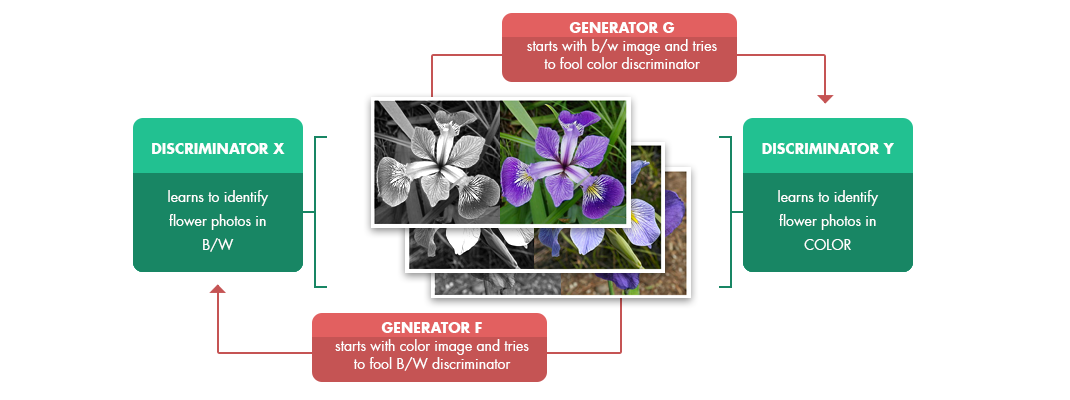
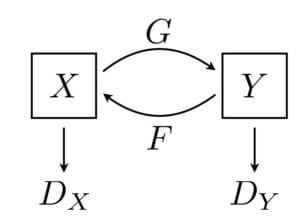
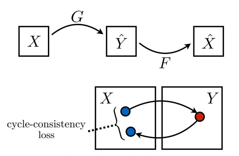
CycleGANs
The Code
Input Pipeline
- trainA: train images for the class A (for example, sunny beach)
- trainB: train images for the class B (for example, cloudy beach)
- testA: class A test images
- testB: class B test images
 real_X = Images(args.input_prefix + '_trainA.tfrecords', batch_size=BATCH_SIZE, name='real_X').feed()
 real_Y = Images(args.input_prefix + '_trainB.tfrecords', batch_size=BATCH_SIZE, name='real_Y').feed()
Generator and discriminator
In this section, we will go more into implementation details depth assuming the reader has some familiarity with how to build CNNs in TensorFlow.
The training graph and main training routines are defined in cyclegan.py (for network architecture details refer to the original paper by Jun-Yan Zhu). The generator is defined in the “generator” function:
def generator(image, norm='batch', rnorm='instance', reuse=False, name="generator")
This network contains two stride-2 convolutions, several residual blocks [14], and two fractionally-strided convolutions with stride 1 2 .
All nonresidual convolutional layers are followed by batch normalization and ReLU nonlinearities with the exception of the output layer, which instead uses a scaled tanh to ensure that the output has pixels in the range [0, 255].
 # define stride-2 convolutions
 s = 256
 c = tf.pad(image, [[0, 0], [3, 3], [3, 3], [0, 0]], "REFLECT")
 c = tf.nn.relu(do_norm(conv2d(c, 32, 7, 1, padding='VALID', name='g_e1_c', reuse=reuse), norm, name + 'g_e1', reuse))
 c2 = tf.nn.relu(do_norm(conv2d(c, 64, 3, 2, name='g_e2_c', reuse=reuse), norm, 'g_e2', reuse))
 c3 = tf.nn.relu(do_norm(conv2d(c2, 128, 3, 2, name='g_e3_c', reuse=reuse), norm, 'g_e3', reuse))
 # define 9 resnet blocks
 r1 = residual_block(c3, 128, norm=rnorm, name='g_r1', reuse=reuse)
 r2 = residual_block(r1, 128, norm=rnorm, name='g_r2', reuse=reuse)
 ...
 r9 = residual_block(r8, 128, norm=rnorm, name='g_r9', reuse=reuse)
 # deconvoutions to size up the image back
 d1 = deconv2d(r9, 64, 3, 2, name='g_d1_dc', reuse=reuse)
 d1 = tf.nn.relu(do_norm(d1, norm, 'g_d1', reuse))
 d2 = deconv2d(d1, 32, 3, 2, name='g_d2_dc', reuse=reuse)
 d2 = tf.nn.relu(do_norm(d2, norm, 'g_d2', reuse))
 d2 = tf.pad(d2, [[0, 0], [3, 3], [3, 3], [0, 0]], "REFLECT")

 # output layer with scaled tanh
 pred = conv2d(d2, 3, 7, 1, padding='VALID', name='g_pred_c', reuse=reuse)
 pred = tf.nn.tanh(do_norm(pred, norm, 'g_pred', reuse))
Loss functions
Generator Loss
Part 1:
 g_loss_G_disc = tf.reduce_mean((discY_fake - tf.ones_like(discY_fake)) ** 2)
 g_loss_F_dicr = tf.reduce_mean((discX_fake - tf.ones_like(discX_fake)) ** 2)
Note: the “**” symbol above is the power operator in Python.
Part 2:
g_loss_G_cycle = tf.reduce_mean(tf.abs(real_X - genF_back))
               + tf.reduce_mean(tf.abs(real_Y - genG_back))
g_loss_F_cycle = tf.reduce_mean(tf.abs(real_X - genF_back))
               + tf.reduce_mean(tf.abs(real_Y - genG_back))
Note: the “” symbol in this context (Python) means that statement spans several lines.
g_loss_G = g_loss_G_disc + g_loss_G_cycle
We used an L1_lambda constant for this multiplier (in the paper the value 10 was used).
g_loss_G = g_loss_G_disc + L1_lambda * g_loss_G_cycle
g_loss_F = g_loss_F_disc + L1_lambda * g_loss_F_cycle
Discriminator Loss
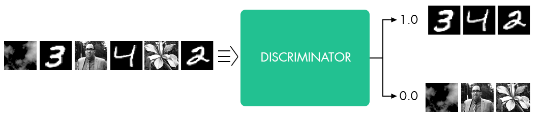
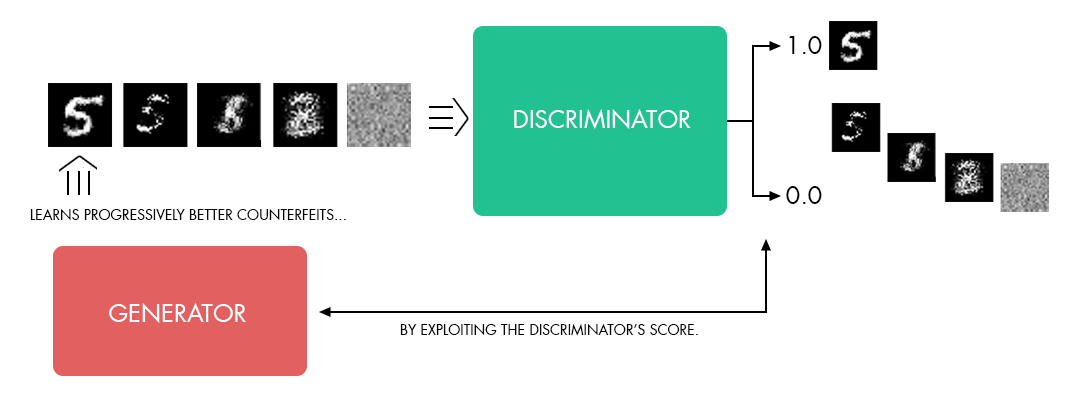
The Discriminator has 2 decisions to make:
- Real images should be marked as real (recommendation should be as close to 1 as possible)
- The discriminator should be able to recognize generated images and thus predict 0 for fake images.
DY_loss_real = tf.reduce_mean((DY - tf.ones_like(DY))** 2)
DY_loss_fake = tf.reduce_mean((DY_fake_sample - tf.zeros_like(DY_fake_sample)) ** 2)
DY_loss = (DY_loss_real + DY_loss_fake) / 2

DX_loss_real = tf.reduce_mean((DX - tf.ones_like(DX)) ** 2)
DX_loss_fake = tf.reduce_mean((DX_fake_sample - tf.zeros_like(DX_fake_sample)) ** 2)
DX_loss = (DX_loss_real + DX_loss_fake) / 2
Training and Results
import numpy as np
import cv2

SPEED = 25
cap = cv2.VideoCapture('./source/beach/beachvideo.mp4')

capture_run = np.random.randint(1000)
totalFrames = 0

def capture_square(frame, square_size, capture_run, totalFrames):
     startX = np.random.randint( int((w-square_size)) )
     startY = np.random.randint( int((h-square_size)) )
     capture = frame[startY:startY+square_size, startX:startX+square_size]
     cv2.imwrite("./captures/cap{0}_f{1}.jpg".format(capture_run, totalFrames),
     capture, [int(cv2.IMWRITE_JPEG_QUALITY), 90])
     totalFrames = totalFrames+1

while(cap.isOpened()):
     ret, frame = cap.read()
     h, w, c = frame.shape
     cv2.imshow('frame', frame)

     if (h < 600) or (w < 600):
          print("width or height of video must be at least 600px")
          break

     key = cv2.waitKey(SPEED)

     # CAPTURE FRAMES WHEN SPACE IS PRESSED
     if key == 32:
          square_size = 600
          capture_square(frame, square_size, capture_run, totalFrames)
          totalFrames = totalFrames + 1

     # QUIT ON 'Q'
     if key == ord('q'):
          break

cap.release()
cv2.destroyAllWindows()
For our task, this approach didn’t deliver a better quality result than the superior images we had access to from Getty Images. However, it provides an interesting avenue for additional CycleGAN projects and we may return to it as a training data source in the future.
Once we had a stable model and good set of training data image sets, we began running various training sessions overnight leveraging both local machines and Azure VM instances to compare various runs concurrently.
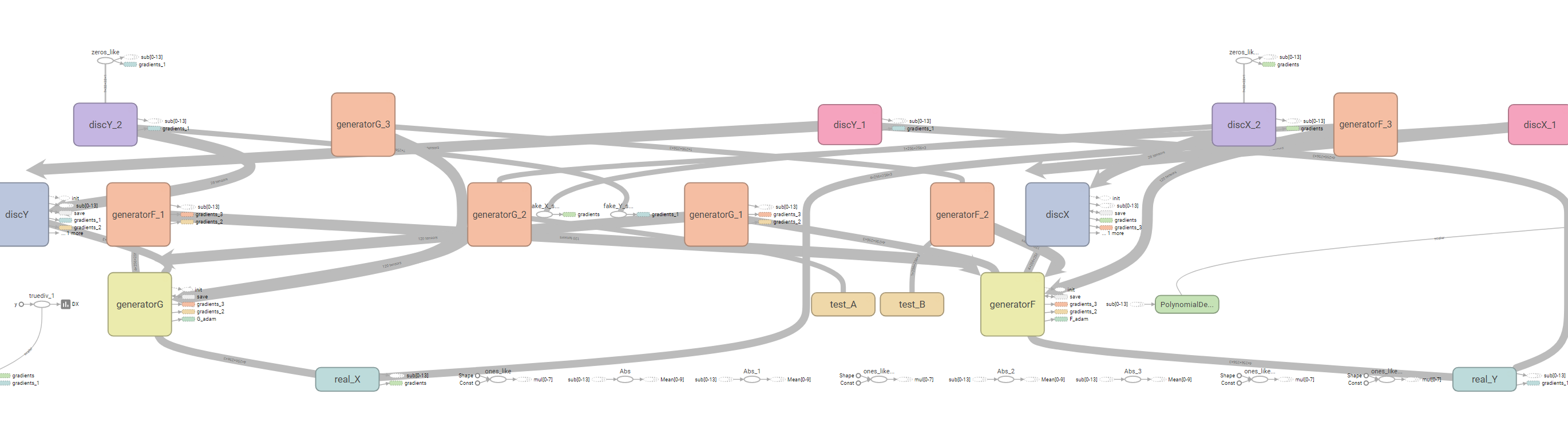
During the run, we would periodically check with TensorBoard to see how well our model was doing. TensorBoard proved invaluable for monitoring our model. However, it seemed to struggle with graphing the model itself, so CycleGANs might be a bit much for it:
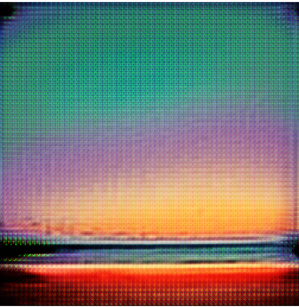
We set up TensorBoard variables that allowed us to monitor not only our loss functions, learning rate decay, and other important parameters but also provided us with glimpses into the images being generated by our model. During training these varied from bizarre to strangely beautiful before settling down to results that looked closer to our goal. Here’s an example of an exotic sunset from one of our runs:
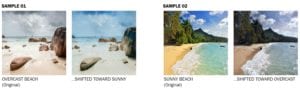
Even if we could never generate photorealistic results, we could at least generate science fiction book covers! Here is a cherry-picked sample of our results at the end of the hackfest, showing that in many cases we approached our goal.
While some of the results were very impressive, there are further optimizations we would like to explore in the future. Additional GANs can be supplemented to help clean up various artifacts created in the process, as well as to allow us to have better resolution while improving the output size. There are also traditional post-processing techniques that can be applied which don’t require deep learning and can improve the aesthetic quality and color balance of the images, which would be valuable if this approach eventually moves toward production quality.
Conclusion
Generative Adversarial Networks are at the forefront of Deep Learning research right now, and CycleGANs are one of the newest methods. We love that our team gets the chance to explore the possibilities of this new technology with partners committed to innovation. The impact of this technology on the creative sector is going to be immense, so we’re trying to ensure that we use approaches that augment creative abilities rather than replace them.
Generative Networks such as the one above are almost always shown operating in the visual realm. One reason is the Convolutional/Deconvolutional nature of the networks, but another large contributor is the striking visual impact of the resulting images. However, we see future generative networks operating in other domains (audio, text, gene sequences, etc.) to help us generate new data for training or, with guidance, creating new works. How can we design loss functions for judging the “aesthetics” of these results? Will other generator and discriminator network topologies produce better results in different domains? There are many open questions, and it’s an exciting time to be working in this field.
If you try out our code on GitHub, please let us know and share your results! If you liked this work, please share it — the more people exploring these emerging questions, the faster we’ll solve them which will benefit us all.
Further Reading
Finally, some useful links for further reading:
- arXiv and perhaps, more importantly, the arXiv Sanity Preserver, for keeping up on the research
- GAN Zoo, for keeping up on GANs in the wild
- Original CycleGAN paper
- Image-to-Image Translation article mentioned above
- Great Distill post on checkerboarding artifacts from Deconvolution layers
 Light
Light Dark
Dark
2 comments
olga, rick and michael, have you seen any startups applying this technology to their products?
These are super new technologies, CycleGans paper is literally few month old. I’ve seen some pix2pix apps, for example this one https://play.google.com/store/apps/details?id=com.dneural.drawzee&hl=en