
Training a Machine Learning Classifier for Relation Extraction from Medical Literature
We recently engaged with Miroculus, a startup working in the medical space. Miroculus develops affordable and quick blood tests for the early detection of diseases by detecting levels of microRNAs in a patient’s blood.
The Problem
As part of their solution, Miroculus attempts to identify if certain miRNAs are related to a certain gene or disease. Based on this data they can create and continually update a tool that lets researchers quickly explore the links between miRNA, genes and their relationship to types of disease (such as cancers). While the medical literature contains many research papers regarding the correlation between certain miRNA, genes, and diseases, there is no one centric database that hold that information in an ordered and structured format.
In our project, we focused on the problem of identifying whether there is a relation between miRNAs and genes by analyzing scientific medical documents. Although there could be different type of relations between miRNA and genes, due to the paucity of data, the relation extraction problem was reduced to binary classification of identifying whether the miRNA and gene are related.
The task of identifying relations between entities from unstructured text is known as the task of Relation extraction. Formally, the task receives unstructured textual input and a group of entities and outputs a group of triplets, each triplet in the form of: (First Entity, Second Entity, Relation Type). It is a subtask in the larger task of Information Extraction.
Since we are dealing with binary classification, we would like to build a classifier that will be given a sentence and a pair of entities and will output a score in the range of 0-1, which represents the probability of the two entities being related.
For example, we will be able pass the classifier the sentence “mir-335 regulates BRCA1”, and the entity pair (mir-335, BRCA1), and receive the score 0.9.
The source code for this project, can be found in: https://github.com/CatalystCode/corpus-to-graph-ml.
In the following post, we will describe the different tasks and items that are needed in order to build a relation classifier:
- Building the Data Set
- Text Transformations
- Feature Representations
- Classification Models Evaluation
- Results
- Opportunities for Reuse
Building the Data Set
We used the text of medical articles from two data sources: PMC and PubMed. The text of the papers downloaded from those data sources was then splitted into sentences using the TextBlob library. And each sentence was given as an input to an entity recognition tool, called GNAT in order to extract the names of the miRNAs and genes that appear in the sentence.
One of the most fundamental challenges in the task of relation extraction (or in any machine learning base task), is the existence of labelled data. For our project, no such data was available for us. Luckily, however, we were able to use an approach called “Distant Supervision”.
Distant Supervision
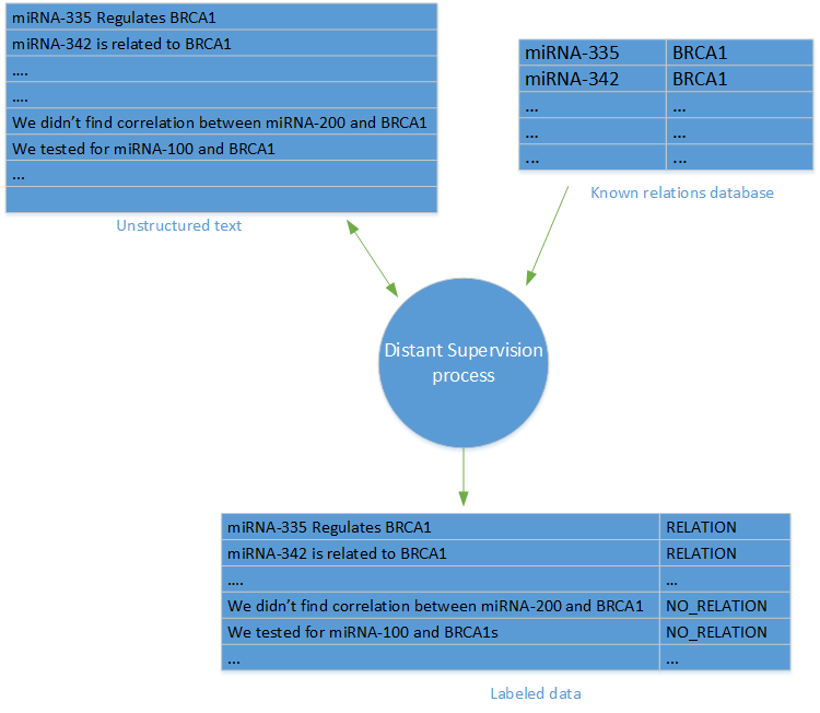
Distant supervision was first used in Distant supervision for relation extraction without labeled data by Mintz et al.. In Distant supervision, a set of labeled data is produced, by leveraging a database of known relations between entities, and a database of articles, containing those entities.
For every pair of entities and a relation from the entities DB, we labeled all of the sentences from the articles DB that contain the entities with the label of the relation.
In order to generate negative samples (that represents no relation), we randomly sampled sentences with entities that do not appear in the relations DB. It’s worth noting that the major caveat of distant supervision is the possible inaccuracy of the negative samples, as we can expect some of the random sampled data to have false negatives.
Text transformations
After we created the labeled training set, we built a relation classifier using scikit-learn Python library, using several NLP based python libraries. We experimented with several possible features and classifiers.
Before trying out several approaches and features, we run the data through a text transformation pipeline, which consists of the following parts:
Entity replacement:
The idea here is that we don’t want the model to learn according to a specific entity name, but we want it to learn according to the structure of the text.
For example:
miRNA-335 was found to regulate BRCA1
Will be transformed to:
ENTITY1 was found to regulate ENTITY2
In practice, we took all pairs of entities in every sentence, and for each pair we replaced the entities in question with place-holders, with ENTITY1 always being a replacement for a miRNA, and ENTITY2 being a replacement for a gene. We used another special placeholder to mark entities that are part of the sentence but are not part of the relation in question.
So, for the following sentence:
High levels of expression of miRNA-335 and miRNA-342 were found together with low levels of BRCA1
We obtained the following set of transformed sentences:
High levels of expression of ENTITY1 and OTHER_ENTITY were found together with low levels of ENTITY2
High levels of expression of OTHER_ENTITY and ENTITY1 were found together with low levels of ENTITY2
This step can be easily implemented by the python string.replace() method in order to replace the entities, and by the itertools.combinations or itertools.product methods in order to walk through all of the possible combinations.
Tokenization
Tokenization is the process of splitting up a sequence of words into smaller segments. In our case, splitting up the sentence into words. We used the nltk library in order to do that:
import nltk
tokens = nltk.word_tokenize(sentence)
Trimming
Following the best practices in the literature, we have trimmed down each sentence to a smaller segment that contains the 2 entities, the words between the entities, and a few words before and after. The purpose of the trimming operation is to remove the parts of the sentence that aren’t relevant to the relation extraction.
In order to do that – we sliced the tokenized array of words from the previous step with the appropriate indices:
WINDOW_SIZE = 3
# make sure that we don't overflow but using the min and max methods
FIRST_INDEX = max(tokens.index("ENTITY1") - WINDOW_SIZE , 0)
SECOND_INDEX = min(sentence.index("ENTITY2") + WINDOW_SIZE, len(tokens))

trimmed_tokens = tokens[FIRST_INDEX : SECOND_INDEX]
Normalization
We normalized the sentences by simply transforming them to lower case. While casing might actually be of value in tasks like sentiment or emotion analysis, it does not play a role in relation extraction, since we are interested in the information and the structure of the text and not on the emphasis of the different words in the sentence.
Stop words / digits removal
Here, we use the common process of removing stop words and digits from the sentence. Stop words are words that occur very often, such as “to” or “is”. As these words occur very often, they do not add much information regarding the relation between the entities in the sentence. For the same reason, we also removed tokens that consisted only of digits, and short token that had no more than 2 characters.
Stemming
Stemming is the process of reducing a given word to its root form. As a result, it reduces the size of the word space, and let us focus on the actual meaning of the word. In practice, we did not find this part to be beneficial for us in terms of accuracy improvements. Because of that and due to the relatively low performance of the process (in terms of run-time), stemming was not included in the final model that was used.
Normalization, words removal and stemming are easily implemented by iterating through the tokenized and trimmed sentence, normalizing and removing words as needed:
cleaned_tokens = []
porter = nltk.PorterStemmer()

for t in trimmed_tokens:
    normalized = t.lower()
    if (normalized in nltk.corpus.stopwords.words('english')
        or normalized.isdigit() or len(normalized) < 2):
        continue
    stemmed = porter.stem(t)
    processed_tokens.append(stemmed)
Feature Representations
After running the transformations above, we were all set up to experiment with different types of features. We’ve experimented with 3 types of features: bag of words, syntactic features, and word embeddings, all explained below:
Bags-of-words
The Bag-of-words model (or just BOW) is a very common and popular method used in NLP based tasks to transform texts into a numerical vector space.
In the BOW model, each word in our vocabulary is assigned to a unique numerical Id. Each sentence is then transformed to a vector in the size of the vocabulary. A position in the vector has the value 1 in case that the word with that id is in the text, or 0 otherwise. An alternative approach is to have each item in the vector hold the number of occurrences for the word in the text. See an example – here.
However, the model described above does not take into account the order of the different words in the sentence, but only the occurrence of each word separately. In order to incorporate the order of the words into the model, we use the popular n-gram model approach, which looks at consecutive words series of length n and treat each series of size n as a different word.
For more information about using n-grams for text analysis, please refer to: “Feature Representation for Text Analyses: 1-gram, 2-gram, 3-gram, but just how many?”.
Luckily for us, the BOW and n-gram models are implemented in scikit-learn by the CountVectorizer class.
The following example transforms the given text to a 1/0 BOW representation with a 3-gram model:
from sklearn.feature_extraction.text import CountVectorizer
vectorizer = CountVectorizer(analyzer = "word", binary = True,
                             ngram_range=(3,3))

# note that 'samples' should be a list/iterable of strings
# so you might need to convert the processes tokens back to sentence
# by using " ".join(...)

data_features = vectorizer.fit_transform(samples)
Syntactic-based features
We used two types of syntactic based features: Part of Speech (POS) Tags, and Dependency Parse Trees.
We have chosen to use https://spacy.io in order to extract both POS tags and dependency graphs, as it seems to outperform existing python libraries in terms of speed with accuracy which is comparable to other NLP frameworks.
The following code snippet, will extract the POS for a given sentence:
from spacy.en import English
parser = English()
parsed = parser(" ".join(processed_tokens))
pos_tags = [s.pos_ for s in parsed]
After transforming each sentence, we can use the CountVectorizer object described above and use a similar Bag-Of-Words model for the POS tags in order to transform them to a numerical vector space.
A similar approach was used for the dependency parse tree features, for which we looked at the path between the 2 entities for each sentence, and transformed it using CountVectorizer as well.
Word embeddings
A recent popular approach in NLP problems is that of word embeddings. The gist of the method is to use neural models in order to transform word to feature space such that similar words will be represented by vectors with small distance between one another.
(Check out this blog post for more information about word embeddings)
We followed the approach presented in Paragraph Vector, which embeds sentences (or documents) in high dimensional feature space. We used the Doc2Vec implementation of the Gensim library. We recommend following this tutorial for more information.
Both the parameters and the size of the output vectors that were used followed the best practices from the Paragraph Vector paper and the Gensim tutorial.
Note that in addition to the labeled data, we also used in our Doc2Vec model a large bunch of additional unlabeled sentences in order to provide more context to the model, and enrich the language and features that the model learns.
After building the model, each sentence was represented by a 200 dimensional vector that can be easily used as an input to the classifier.
Classification Models Evaluation
Once the text transformations and feature extraction are completed, the next step is to select, and then evaluate our classification model.
The algorithm that was used for the classification part was Logistic Regression. We also tried other algorithms like SVM and Random Forest, but Logistic Regression outperformed those in terms of speed and accuracy.
Before starting to evaluate the accuracy of the method, we first need to split our dataset into a training set and a test set. This is done easily using the train_test_split method:
from sklearn.cross_validation import train_test_split
x_train, x_test, y_train, y_test = train_test_split(data, labels, test_size=0.25)
This will split the data set randomly, with 75% of the data split to the training set and 25% to the test set.
To train a classifier using Logistic Regression, we use the scikit-learn LogisticRegression class. To understand how well the classier is performing we use the classification_report class, which prints the precision, recall, and F1-Score of the classification.
The following code snippet trains a logistic regression classifier and prints a classification report:
from sklearn.linear_model import LogisticRegression
from sklearn.metrics import classification_report

clf = linear_model.LogisticRegression(C=1e5)
clf.fit(x_train, y_train)
y_pred = clf.predict(x_test)
print classification_report(y_test, y_pred)
A sample output of the code snippet above will look something like this: “`python
  precision    recall  f1-score   support

      0       0.82      0.88      0.85      1415
      1       0.89      0.83      0.86      1660

avg / total   0.86      0.85      0.85      3075
Note that the C parameter (which stands for the regularization strength) is chosen arbitrarily for this example, but should be tuned using cross validation, as mentioned below.
Results
We combined all of the methods and techniques described above and compared the different features and transformations in order to choose the model that works best for us.
We have used the LogisticRegressionCV class to build a binary classifier with tuned parameters, and then evaluated a different test set in order to evaluate the model performance. Note that for testing different parameters of different features easily, you can use the GridSearch class.
The table below lists the top results of comparing the different features that we’ve tried. We have used the F1-Score as an accuracy measurement for our model, as it captures both the accuracy and the recall of the model.
| Features | F1-Score |
|---|---|
| Bag-Of-Words 1-3 Gram | 0.87 |
| BOW 1-3 Grams and POS Tags 3 Gram | 0.87 |
| BOW 1-3 Grams and Doc2Vec | 0.87 |
| Bag-Of-Words 1 Gram | 0.8 |
| Bag-Of-Words 2 Gram | 0.85 |
| Bag-Of-Words 3 Gram | 0.83 |
| Doc2Vec | 0.65 |
| POS Tags 3 Grams | 0.62 |
In general, it seems that using Bag-Of-Words of 1-to-3 n-grams prevails over the other approaches and achieves the best accuracy. While the Doc2Vec model seem to excel at tasks like words similarity, it does not perform as well for relation extraction.
Opportunities for Reuse
In this post, I presented the approach that we took for building an entity relation classifier for relations between miRNA and genes.
While the problem and examples shown here are related to the biological domain, the solution and approaches mentioned above can be applied to other domains in order to build a graph of relations using unstructured textual data.
 Light
Light Dark
Dark
0 comments